A short history of the standard deviation
The standard deviation was in use for most of a century before it had its name. It started as a tool for astronomers trying to decide how far to trust a measurement, went by several names and several rival definitions, and settled into its modern form only around 1900.
┄ ±1 probable error (±0.5″, 0.6745σ): middle 50% ━ ±1σ (±0.741″): middle 68.3%
Astronomers and their errors
In the 18th century the pressing statistical problem was not describing populations but combining observations. An astronomer measuring the position of a planet several times got several slightly different answers and had to decide what the true value was and how much to trust it. Two ideas from this period still sit underneath every standard deviation.
The first is the bell-shaped curve. Abraham de Moivre derived it in 1733 as an approximation to the binomial distribution, the probabilities of getting a given number of heads in many coin tosses. The second is least squares. Adrien-Marie Legendre published the method in 1805: choose the answer that makes the sum of squared differences from the observations as small as possible. Squared differences are the raw material of the standard deviation, and least squares is why squaring, rather than taking absolute values, became the standard choice.
Carl Friedrich Gauss connected the two in 1809, in his book on the motion of heavenly bodies (Theoria motus corporum coelestium). He showed that if measurement errors follow the bell curve, least squares gives the most probable answer. This is why the normal distribution is still sometimes called the Gaussian distribution, and why the standard deviation and the normal curve are so closely linked. Pierre-Simon Laplace's work on what is now called the central limit theorem, around 1810, explained why so many kinds of error should follow that curve.
Many names for one spread
Once errors were understood as following a curve, astronomers needed a single number for how wide the curve was. Throughout the 19th century they used several, all proportional to what we now call σ:
| Measure | Definition, for normal errors | In units of σ |
|---|---|---|
| Mean error (Gauss) | Square root of the mean squared error | 1 |
| Probable error | Half the errors are smaller than this | 0.6745 |
| Mean absolute error | Average size of an error, ignoring sign | 0.7979 |
| Modulus | The width parameter in the curve's exponent | 1.4142 |
Gauss's mean error is the standard deviation under another name. In the 1820s, in his later work on combining observations, he adopted it as his measure of precision and also dealt with the fact that errors measured from an estimated value run slightly small, the problem that the n − 1 divisor corrects. (That divisor is now usually called Bessel's correction, after the astronomer Friedrich Bessel; the reasons for dividing by n − 1 are set out on the sample vs population page.)
In practice, though, the most quoted measure for most of the century was the probable error. It had an intuitive meaning, an even bet that the true error is smaller, and it appears in astronomy, geodesy and early biometrics well into the 1900s.
Worked example: reading an old probable error
Anyone reading a 19th-century measurement today has to convert. Suppose an old paper reports a star's position with a probable error of ±0.5 arcseconds. The probable error is the point that cuts off the middle 50% of a normal curve, which is z = 0.6745 (the 75th percentile of the standard normal distribution; the inverse normal calculator gives it). So:
σ = probable error / 0.6745 σ = 0.5 / 0.6745 = 0.741 arcseconds
The same measurement expressed in the other old units would have been a mean absolute error of 0.741 × 0.7979 = 0.591 and a modulus of 0.741 × 1.4142 = 1.048. Four numbers, one spread. A modern reader who took the probable error for a standard deviation would understate the uncertainty by about a third, since 0.5 is 67% of 0.741.
The interpretations differ too. About 50% of errors fall within ±1 probable error, and about 68.3% within ±1 standard deviation. The second figure is the start of the 68–95–99.7 rule.
Try it: inverse normal distribution calculator
The calculator below opens on its own defaults; enter an area of 0.75 with mean 0 and standard deviation 1 to recover the 0.6745 behind the probable error, or put in your own numbers.
Between 0 and 1, e.g. 0.95 or 95%.
Use μ = 0 and σ = 1 for a z-score.
The curve is the probability density; the shaded area is the probability asked for.
| Left-tail area | z | x |
|---|---|---|
| 0.9 | 1.2816 | 119.223 |
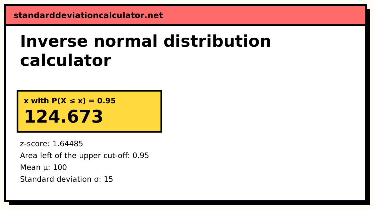
| 0.95 | 1.6449 | 124.673 |
| 0.975 | 1.96 | 129.399 |
| 0.99 | 2.3263 | 134.895 |
| 0.995 | 2.5758 | 138.637 |
Show the working, step by step
Turn the area into the probability to the left of a cut-off.
The area to the left is the probability itself: 0.95.
Find z from the inverse standard normal CDF:
z = Φ⁻¹(0.95) = 1.64485
Convert z back to the scale of X:
x = μ + zσ = 100 + 1.64485 × 15 = 124.673
Φ⁻¹ is evaluated with Acklam’s rational approximation, accurate to about 1 part in a billion.
Open the full inverse normal distribution calculator for two-tailed areas and more worked examples.
Pearson names it, 1893–1894
The name "standard deviation" comes from Karl Pearson, the English mathematician who, with Francis Galton and W. F. R. Weldon, built the biometric school of statistics in London. He introduced the term in lectures in 1893 and used it in print in 1894, in the first of his papers titled "Contributions to the Mathematical Theory of Evolution" in the Philosophical Transactions of the Royal Society. That paper also wrote it with the Greek letter σ.
The new name did not describe a new quantity. It was Gauss's mean error, applied to variation among living things rather than to measurement errors. That change of subject is the real shift. For the astronomers, spread was a nuisance to be minimised. For Pearson and the biometricians, the spread of heights, skull sizes or crab measurements in a population was itself the thing being studied, and "error" was the wrong word for it.
Student, Fisher and variance
Two further steps made the standard deviation what it is in a modern textbook. In 1908 William Sealy Gosset, writing as "Student" in the journal Biometrika, published "The probable error of a mean". It worked out how to handle the uncertainty in a mean when the standard deviation itself has to be estimated from a small sample, which led to the t distribution. The paper's title shows the probable error was still the working vocabulary.
In 1918 Ronald Fisher, in a paper on the correlation between relatives under Mendelian inheritance, introduced the word "variance" for the square of the standard deviation. His reason was practical: variances from independent causes add, standard deviations do not, which makes the square the easier quantity to break into parts. That idea became the analysis of variance. The relationship between the two measures is covered in standard deviation vs variance.
Timeline
| Year | Event |
|---|---|
| 1733 | De Moivre derives the normal curve as an approximation to the binomial |
| 1805 | Legendre publishes the method of least squares |
| 1809 | Gauss links least squares to the normal law of errors |
| 1820s | Gauss's later work treats the mean error, the modern σ |
| 1893 | Pearson introduces the term "standard deviation" in lectures |
| 1894 | Pearson uses "standard deviation" and σ in print |
| 1908 | Student's paper on the probable error of a mean |
| 1918 | Fisher names the square of the SD "variance" |
The standard deviation won out over its rivals for reasons that are all visible in this history: it is the natural partner of least squares and the normal curve, it squares neatly into the variance, and variances add. The probable error had the friendlier meaning, but the standard deviation had the better algebra.
Related calculators
-
What is standard deviation?
The modern idea, explained with examples.
-
Standard deviation and the normal distribution
The curve the SD was first built around.
-
Standard deviation symbol
σ, s and the other notations in use today.
Common questions
Who invented the standard deviation?
No single person. The quantity, the square root of the mean squared error, was in use by Gauss and other astronomers in the early 19th century under names such as "mean error". Karl Pearson gave it the name "standard deviation" in 1893 and used it in print in 1894.
Why is the standard deviation written σ?
Pearson used the Greek lower-case sigma for it in his 1894 paper, and the notation stuck. Today σ usually denotes the population value and s the sample estimate. The standard deviation symbol page covers the conventions in use now.
What was the probable error?
The half-width of the interval that contains half of all errors, for normally distributed errors. It equals 0.6745 standard deviations. It was the usual way to quote precision for most of the 19th century and survived in some fields well into the 20th, before the standard deviation replaced it.