The standard deviation of proportions
Survey answers, conversion rates, pass rates and defect rates are all proportions: counts of yes out of a total. Proportions have a standard deviation like any other data, and it follows a short formula that explains why polls quote the margins of error they do.
Yes/no data is just 0s and 1s
Code each yes as 1 and each no as 0. The mean of those numbers is the proportion of yeses. Suppose ten people answer a question and seven say yes:
1, 1, 1, 1, 1, 1, 1, 0, 0, 0
The mean is 7 ÷ 10 = 0.7. Now take the standard deviation of those ten numbers in the usual way. Seven values are 0.3 above the mean and three are 0.7 below it:
σ² = [7 × 0.3² + 3 × 0.7²] / 10 = [0.63 + 1.47] / 10 = 0.21 σ = √0.21 = 0.458
Notice that 0.21 is 0.7 × 0.3. That is not a coincidence. For any list of 0s and 1s with a proportion p of 1s, a fraction p of the values sit at distance 1 − p above the mean and a fraction 1 − p sit at distance p below, so the variance is p(1 − p)² + (1 − p)p², which simplifies to p(1 − p):
σ = √(p(1 − p))
That is the population version, dividing by n. If you paste the ten values into the standard deviation calculator in sample mode you will get 0.483 instead, which is √(0.21 × 10 ÷ 9); the n − 1 correction matters for ten values and fades for large samples. The same result appears as the standard deviation of a Bernoulli random variable on the standard deviation in probability page.
Why it peaks at p = 0.5
The formula depends on nothing but p, so you can tabulate it once:
| p (or 1 − p) | p(1 − p) | SD √(p(1 − p)) |
|---|---|---|
| 0.01 (0.99) | 0.0099 | 0.099 |
| 0.1 (0.9) | 0.09 | 0.300 |
| 0.2 (0.8) | 0.16 | 0.400 |
| 0.3 (0.7) | 0.21 | 0.458 |
| 0.4 (0.6) | 0.24 | 0.490 |
| 0.5 | 0.25 | 0.500 |
The largest possible SD for yes/no data is 0.5, reached when the split is even. Algebraically, p(1 − p) = 0.25 − (p − 0.5)², so it is 0.25 minus a square that is zero only at p = 0.5. Intuitively, a 50/50 split is the least predictable: if you had to guess one person's answer you would be wrong half the time. When 99% say yes, almost everyone gives the same answer and there is very little spread.
The curve is also flat near the top. Between p = 0.3 and p = 0.7 the SD only ranges from 0.458 to 0.5, which is why planning a survey for the worst case costs little when the true answer turns out to be anywhere in the middle.
From SD to the standard error of a proportion
A survey reports the sample proportion p̂, which is the mean of the 0s and 1s. Like any sample mean, its standard error is the SD divided by √n:
SE(p̂) = √(p(1 − p) / n)
The SD tells you how much individual answers differ; the SE tells you how much the proportion would move if you repeated the whole survey with a fresh sample. More respondents do not make people agree with each other more, so the SD stays put, but they do pin down the proportion more precisely, so the SE shrinks. The p-hat calculator gives p̂ and its standard error from a count and a total.
Worked example: a survey of 400
A hypothetical company surveys 400 customers and 120 say they would recommend it. Then:
p̂ = 120 / 400 = 0.30 SD = √(0.30 × 0.70) = 0.458 SE = √(0.21 / 400) = 0.0229 95% MOE = 1.96 × 0.0229 = 0.0449 95% CI = 0.30 ± 0.045 = 0.255 to 0.345
The result is 30% with a margin of error of about 4.5 percentage points, so the true share is plausibly anywhere from about 25.5% to 34.5%. The margin of error calculator runs the same steps. The check that the normal approximation is reasonable: 120 successes and 280 failures, both well over 10.
Try it: p-hat calculator
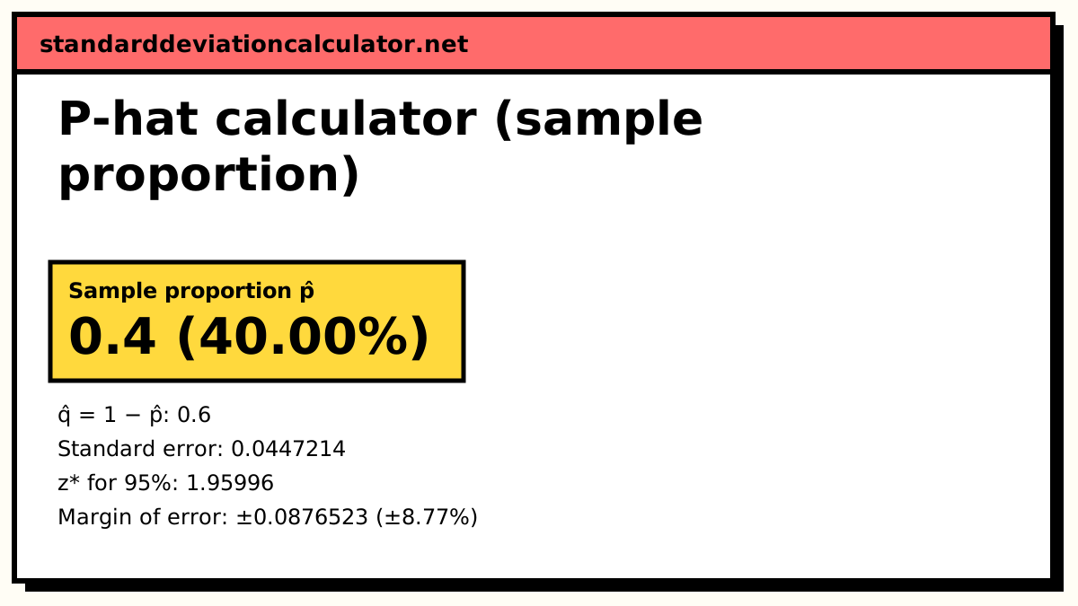
The calculator opens with its own example of 48 successes out of 120; enter x = 120 and n = 400 to reproduce the survey above, or your own count and total.
How many in the sample have the trait.
Show the working, step by step
Divide the successes by the sample size.
p̂ = x ÷ n = 48 ÷ 120 = 0.4
Standard error of p̂:
SE = √(p̂(1 − p̂) ÷ n) = √(0.4 × 0.6 ÷ 120) = 0.0447214
Margin of error at 95% confidence:
E = z* × SE = 1.95996 × 0.0447214 = 0.0876523
Confidence interval:
p̂ ± E = 0.4 ± 0.0876523 = (0.312348, 0.487652)
Check the conditions for the normal approximation.
n·p̂ = 48 ≥ 10, n·(1 − p̂) = 72 ≥ 10
The Wilson interval adds z²/2n to the successes before centring, which keeps it inside 0 to 1 and gives better coverage when p̂ is near 0 or 1.
Open the full p-hat calculator for the Wilson interval and when to use it.
How sample size changes the margin
Because p(1 − p) is at most 0.25, the widest 95% margin of error for a given n is 1.96 × √(0.25 ÷ n). This is the figure pollsters quote:
| Sample size n | Max 95% margin of error |
|---|---|
| 100 | ±9.8 points |
| 400 | ±4.9 points |
| 1,000 | ±3.1 points |
| 2,500 | ±2.0 points |
Quadrupling the sample halves the margin, since n sits under a square root. Going from 400 to 1,600 respondents buys the same improvement as going from 100 to 400, at four times the cost. The sample size calculator works this backwards from the margin you want.
Our survey of 400 had a margin of 4.5 points rather than the table's 4.9 because 0.3 × 0.7 = 0.21 is a little below 0.25. For rare outcomes the gap is large: at p = 0.01 with n = 400, the formula's SE is only 0.005. But 1% of 400 is four people, too few for the normal approximation, and an interval built from it can even dip below zero. The FAQ below covers what to do instead.
Common mistakes
Using the SD where the SE belongs. Writing “30% ± 0.458” confuses the variation between people with the uncertainty in the percentage. The ± on a survey result should come from the standard error.
Applying the margin of error to subgroups. A poll of 1,000 has a margin of about 3 points overall, but if 200 of the respondents are under 30, the margin for that group alone is about 1.96 × √(0.25 ÷ 200) = 6.9 points.
Forgetting that the formula only covers sampling error. Non-response, leading questions and an unrepresentative sample add error that no √n can shrink.
Related calculators
-
P-hat calculator
Sample proportion, its standard error and a confidence interval.
-
Margin of error calculator
The ± figure for a survey result, for a mean or a proportion.
-
Sampling distribution of p̂
Probabilities for a sample proportion, with the working.
Common questions
What is the difference between the SD of the data and the standard error of a proportion?
The SD, √(p(1 − p)), describes how much individual yes/no answers vary, and it does not shrink as you collect more data. The standard error, √(p(1 − p) ÷ n), describes how much the sample proportion would vary from one sample to the next, and it falls as n grows. Polls and confidence intervals use the standard error.
Why do pollsters use p = 0.5 when planning a survey?
Because p(1 − p) is largest at 0.5, so assuming 0.5 gives the widest margin of error any result could need. A sample sized for 0.5 is big enough whatever the answer turns out to be. That is where the familiar “about ±3 points with 1,000 people” comes from.
Can I use √(p(1 − p) ÷ n) when p is very close to 0 or 1?
It gets unreliable. The normal approximation behind it needs roughly 10 or more successes and 10 or more failures, and with a rare outcome you often have fewer. A proportion of 0 then gives a standard error of 0, which is plainly wrong. Use a Wilson or exact (Clopper–Pearson) interval instead.