How outliers affect the standard deviation
The standard deviation squares every distance from the mean, so a single value far from the rest can dominate it. This post measures that effect on a small dataset, shows why the influence grows the further out the value sits, and compares the SD with measures of spread that barely notice the outlier at all.
━ Standard deviation ━ IQR ┄ MAD
The starting data
Take ten delivery times, in minutes, from a hypothetical local shop:
12, 14, 15, 15, 16, 17, 18, 18, 19, 20
They sum to 164, so the mean is 16.4 minutes. The sum of squared deviations is 54.4, giving a sample standard deviation of √(54.4 ÷ 9) = 2.46 minutes. The median is 16.5. Nothing unusual: most deliveries take a quarter of an hour, give or take a couple of minutes.
One value, moved further and further out
Now suppose the last delivery was not 20 minutes but was held up: 30 minutes, then 50, then 100, then 200. The other nine values stay the same. Here is what happens to each measure:
| Last value | Mean | SD | Median | MAD | IQR |
|---|---|---|---|---|---|
| 20 | 16.4 | 2.46 | 16.5 | 1.5 | 3.0 |
| 30 | 17.4 | 4.90 | 16.5 | 1.5 | 3.0 |
| 50 | 19.4 | 10.96 | 16.5 | 1.5 | 3.0 |
| 100 | 24.4 | 26.65 | 16.5 | 1.5 | 3.0 |
| 200 | 34.4 | 58.22 | 16.5 | 1.5 | 3.0 |
(IQR by the inclusive quartile method: Q1 = 15, Q3 = 18 in every row.) Changing one delivery from 20 to 30 minutes doubles the standard deviation. At 100 minutes it is more than ten times the original, and it now says a typical delivery is 26 minutes away from the average, when nine of the ten were within 4 minutes of 16. The mean drifts too, but more slowly: each extra minute on the last value adds 0.1 to the mean, one tenth, because it is one value in ten.
Try it: standard deviation calculator
The deliveries are filled in with the last one at 100 minutes; change it to 20, 30 or any other value and watch the standard deviation follow.
Separate numbers with commas, spaces or new lines, or paste a spreadsheet column.
Decimals and negatives are fine; write 10:3 for a value that occurs 3 times.
Your results will appear here: the standard deviation first, then the rest of the summary and a chart.
Standard deviation (sample)
26.6467
26.65
Your values typically sit about 26.6 above or below their mean of 24.4, in the same units as your data. 9 of 10 values (90%) fall between -2.247 and 51.05, within one standard deviation of the mean; for normally distributed data about 68% would.
Population SD (σ): 25.2792, if these values are the whole group.
- Count (n)
- 10
- Mean (x̄)
- 24.4
- Variance (s²)
- 710.044
- Standard error
- 8.42641
- Minimum
- 12
- Q1 (25%)
- 15
- Median
- 16.5
- Q3 (75%)
- 18
- Maximum
- 100
- Range
- 88
More statistics (5)
- Relative SD (%RSD)
- 109.208%
- Coefficient of variation
- 1.09208
- Sum (Σx)
- 244
- Sum of squares, Σ(x − x̄)²
- 6390.4
- IQR (Q3 − Q1)
- 3
Data distribution
Shaded bands mark ±1, ±2 and ±3 SD from the mean. 9 of 10 values (90%) fall within ±1 SD.
Chart as text
Mean 24.4, sample standard deviation s = 26.6467, from 10 values between 12 and 100.
- Within ±1 SD (-2.247 to 51.05): 9 of 10 values (90%). About 68% for normal data.
- Within ±2 SD: 9 (90%). About 95% for normal data.
- Within ±3 SD: 10 (100%). About 99.7% for normal data.
Show the working, step by step
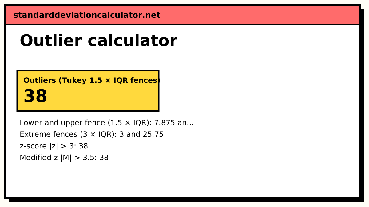
Open the full standard deviation calculator for more examples, or the outlier calculator to test which values are flagged.
Why the influence grows with distance
The mean responds to an outlier in proportion to its distance. The SD responds to the square of the distance, inside a square root, and the square quickly takes over. With the last value at 30, its deviation from the new mean is 30 − 17.4 = 12.6, and 12.6² = 158.76 is 73% of the sum of squares, 216.4. At 100, the deviation is 75.6, its square is 5,715.36, and that one term is 89% of the total of 6,390.4. One value out of ten supplies nearly nine tenths of what the SD is built from.
Once the outlier dominates, the SD grows almost in a straight line with it. From 100 to 200 the last value doubles, and the SD goes from 26.65 to 58.22, slightly more than doubling. The SD has stopped describing the nine ordinary deliveries and is now mostly a measure of how far away the tenth one is.
The masking problem
The obvious way to spot the outlier is its z-score. Here is the catch: the outlier inflates the SD it is being divided by. With the last value at 30, its z-score is (30 − 17.4) ÷ 4.90 = 2.57. At 50 it is 2.79. At 100 and at 200 it is 2.84. It can never exceed (n − 1) ÷ √n, which for ten values is 9 ÷ √10 = 2.85, however extreme the value. A rule of “flag anything more than 3 SDs out” will never catch a single outlier in a sample of ten.
Measures that hold still
The median and the two spreads built on it did not move in any row of the table. They depend on the order of the values, not on how far the largest one is from the rest.
The median absolute deviation is the median of the distances from the median. In the clean data the distances from 16.5 run from 0.5 to 4.5, and their median is 1.5. Multiplied by 1.4826, the MAD estimates what the SD would be for normal data without the contamination: 2.22 minutes, close to the clean SD of 2.46. The matching modified z-score, 0.6745 × (x − median) ÷ MAD, has no ceiling. For the 30-minute delivery it is 0.6745 × 13.5 ÷ 1.5 = 6.07, well past the usual cut-off of 3.5.
The interquartile range is the spread of the middle half of the data, 3.0 minutes here in every row. The Tukey fences put the upper limit at Q3 + 1.5 × IQR = 18 + 4.5 = 22.5, so every variant from 30 upward is flagged, and the clean value of 20 is not.
These measures are not better than the SD in general. For clean, roughly normal data the SD uses more of the information and is more precise. They are better when you suspect contamination, or as a check: if the SD and 1.4826 × MAD disagree by a factor of two or more, look at the extremes before trusting either.
Keep it or remove it?
The statistics can tell you a value is unusual. They cannot tell you whether it belongs. That depends on where it came from.
Remove or correct it when it is an error: a typo (a 200 that should be 20), a sensor fault, a unit mix-up, a test entry, or a case from outside the population you meant to study. Fix it at the source if you can, and note what you changed.
Keep it when it is a real observation. If a delivery really did take 100 minutes, the customer waited 100 minutes. For a shop planning its promises, that late tail is the most important part of the data, and deleting it would make the service look more reliable than it is. In finance, insurance and safety work, the extremes are often the whole point.
When you are unsure, report the result both ways and state what was excluded. Deciding after seeing the numbers which values to drop, and keeping whichever version supports the conclusion you hoped for, is how analyses go wrong. The outlier calculator runs the fences, z-scores and Grubbs’ test side by side so you can see which points are borderline before you decide.
For how the mean and SD compare when an outlier appears, the standard deviation vs mean page has a second worked example. For the SD itself, start with what is standard deviation.
Related calculators
-
Outlier calculator
Tukey fences, z-scores and Grubbs’ test on your own data.
-
Median absolute deviation calculator
MAD and modified z-scores, which one outlier cannot inflate.
-
IQR calculator
The spread of the middle half of the data.
Common questions
Does an outlier always increase the standard deviation?
Adding a value far from the mean always increases it, because its squared deviation is large. Adding a value close to the mean can decrease it slightly, since it adds a small squared deviation while increasing n. Removing a genuine outlier therefore almost always shrinks the SD, often by a lot.
Why did my z-score test miss an obvious outlier?
Because the outlier inflated the standard deviation it was being measured against. In a sample of n values, no single point can have a z-score (using the sample SD) larger than (n − 1) ÷ √n, which is 2.85 for n = 10. A “flag anything beyond 3” rule can never fire on ten values. Use the median and MAD, or the IQR fences, for small samples.
Should I report the SD with or without the outlier?
If the value is an error, correct or remove it and report the SD without it. If it is a real observation, keep it in the main result. When removal is a judgement call, report both and say which values were excluded and why, so a reader can see how much the conclusion depends on that one point.