Sample vs population standard deviation
The two standard deviations differ in one place: the sample version divides by n − 1, the population version by N. Which you should use has nothing to do with how much data you have, and everything to do with what you are trying to describe.
When to use sample vs population standard deviation
Ask: are these numbers the entire group I want to draw a conclusion about?
- Yes, that's all of them → population, divide by N (work out σ for the whole population).
- No, they stand in for something larger → sample, divide by n − 1 (work out s for a sample).
The same dataset can be either. Twelve monthly sales figures are a population if you want the variability of last year, and a sample if you want to estimate how much sales vary in general. Nothing about the numbers changes, only the question.
| Situation | Which | Why |
|---|---|---|
| Survey of 500 people in a city of 900,000 | Sample | Standing in for the city |
| Every test score in one class, describing that class | Population | Nothing is left out |
| Every test score in one class, generalising to the school | Sample | The class stands in for more |
| Six replicate lab measurements | Sample | Estimating what the method would keep doing |
| Daily returns for a stock over its full listed history | Population | That history is complete… |
| …the same returns, used to forecast future volatility | Sample | …but the future is not in it |
| All 50 US state populations from the census | Population | There are exactly 50 |
See the difference on your own data
Enter numbers and switch the mode to compare the two directly.
Separate numbers with commas, spaces or new lines, or paste a spreadsheet column.
Decimals and negatives are fine; write 10:3 for a value that occurs 3 times.
Your results will appear here: the standard deviation first, then the rest of the summary and a chart.
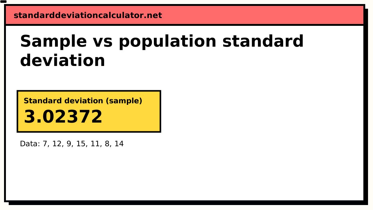
Standard deviation (sample)
3.02372
3.02
Your values typically sit about 3.02 above or below their mean of 10.86, in the same units as your data. 4 of 7 values (57%) fall between 7.833 and 13.88, within one standard deviation of the mean; for normally distributed data about 68% would.
Population SD (σ): 2.79942, if these values are the whole group.
- Count (n)
- 7
- Mean (x̄)
- 10.8571
- Variance (s²)
- 9.14286
- Standard error
- 1.14286
- Minimum
- 7
- Q1 (25%)
- 8.5
- Median
- 11
- Q3 (75%)
- 13
- Maximum
- 15
- Range
- 8
More statistics (5)
- Relative SD (%RSD)
- 27.85%
- Coefficient of variation
- 0.2785
- Sum (Σx)
- 76
- Sum of squares, Σ(x − x̄)²
- 54.8571
- IQR (Q3 − Q1)
- 4.5
Data distribution
Shaded bands mark ±1, ±2 and ±3 SD from the mean. 4 of 7 values (57%) fall within ±1 SD.
Chart as text
Mean 10.8571, sample standard deviation s = 3.02372, from 7 values between 7 and 15.
- Within ±1 SD (7.833 to 13.88): 4 of 7 values (57%). About 68% for normal data.
- Within ±2 SD: 7 (100%). About 95% for normal data.
- Within ±3 SD: 7 (100%). About 99.7% for normal data.
Show the working, step by step
How large is the gap?
The sample variance is always the population variance multiplied by n/(n − 1). The standard deviations therefore differ by the square root of that factor:
| n | Variance is larger by | SD is larger by |
|---|---|---|
| 2 | 100% | 41.4% |
| 5 | 25% | 11.8% |
| 10 | 11.1% | 5.4% |
| 30 | 3.4% | 1.7% |
| 100 | 1.0% | 0.5% |
| 1000 | 0.1% | 0.05% |
Beyond about n = 100 the choice is cosmetic. Below about n = 20 it is not, and small datasets are exactly where people are most likely to be calculating by hand and least likely to have thought about which mode they are in.
Why n − 1 rather than n
Here is the intuition. The sample mean x̄ is calculated from your sample, which means it is positioned to sit as centrally among those particular numbers as it possibly can. The true population mean μ sits somewhere else, and on average slightly further from your data points.
So Σ(x − x̄)² is systematically smaller than Σ(x − μ)² would have been. Not sometimes; always, except in the vanishing case where x̄ happens to land exactly on μ. Dividing by n would inherit that shortfall and understate the population's spread every single time.
The mathematics works out cleanly: the expected value of Σ(x − x̄)² is exactly (n − 1)σ². So dividing by n − 1 rather than n gives an estimator whose long-run average is σ² exactly. That is Bessel's correction.
The n − 1 is also the degrees of freedom. Once you know the mean and n − 1 of the values, the last one is determined: the deviations must sum to zero. Only n − 1 of them are free to vary, and the divisor counts free pieces of information rather than raw data points.
The mistake to watch for
The word "population" appearing in a problem is not evidence. "The standard deviation of the population of fish in the lake, based on a catch of 40" is a sample calculation: 40 fish are not the lake. What matters is whether the numbers in front of you are exhaustive, not what the group is called.
To see both formulas applied to real data sets step by step, work through the standard deviation examples.
Related calculators
-
Standard deviation calculator
Toggle between the two modes and watch the denominator change.
-
The formula explained
Both formulas taken apart term by term.
-
σ vs s notation
The symbols that mark the same distinction.
-
Variance calculator
Where the n − 1 correction is exactly unbiased.
Common questions
Should I use sample or population standard deviation?
Use population only if your numbers are the complete group you want to describe, with nothing left out. Use sample in every other case: whenever the numbers are a subset being used to say something about a wider group.
Sample is correct far more often in practice. If you genuinely cannot decide, choose sample: it produces the slightly larger, more conservative estimate.
How much difference does the choice make?
The sample variance is always larger by a factor of n/(n − 1). With n = 5 that is 25%; with n = 30 it is 3.4%; with n = 1000 it is 0.1%. The standard deviations differ by the square root of those factors, so the effect is smaller still, but on small datasets it is easily large enough to change a conclusion.
Is a class of 30 students a population or a sample?
Both, depending on your question. If you want to describe that class (the mean score in Period 3), the 30 students are the population. If you want to use them to say something about students in general, or about how the class would do on a different test, they are a sample.
The data does not decide this. Your question does.
Which one does Excel use by default?
STDEV() and STDEV.S() are the sample version; STDEV.P()
is the population version. The plain STDEV(), the one people reach for
without thinking, is the sample version, which is usually the right default.
Why does dividing by n − 1 fix the bias?
A sample's mean is computed from that sample, so it sits closer to those specific points than the true population mean does. Spread measured around it is therefore too small every time, not just sometimes. The expected value of Σ(x − x̄)² turns out to be exactly (n − 1)σ², so dividing by n − 1 rather than n makes the estimate unbiased by construction.
Note the correction is exactly unbiased for the variance. Because the square root is a non-linear function, s is still very slightly biased as an estimate of σ, a subtlety that almost never matters in practice.
Questions about sample vs population standard deviation
Common questions
Can I convert sample standard deviation to population standard deviation for a quality-control sample?
Use the sample standard deviation (divide by n − 1) when your data is a subset of a larger group, which covers nearly every real dataset. Use the population standard deviation (divide by N) only when your data includes every member of the group. The n − 1 correction (Bessel's correction) compensates for the fact that a sample's own mean is always closer to its values than the true population mean. See sample vs population standard deviation for a full guide with examples.
What sample size is needed to estimate standard deviation for a class test?
Standard deviation is a measure of how spread out a set of numbers is around their mean. It is the square root of the average squared distance from the mean, expressed in the same units as the original data. A small standard deviation means values cluster close to the mean; a large one means they are widely scattered. See what is standard deviation for a full explanation with examples.
What sample size is needed to estimate standard deviation for a survey?
Standard deviation is a measure of how spread out a set of numbers is around their mean. It is the square root of the average squared distance from the mean, expressed in the same units as the original data. A small standard deviation means values cluster close to the mean; a large one means they are widely scattered. See what is standard deviation for a full explanation with examples.
What sample size is needed to estimate standard deviation for a quality-control sample?
Standard deviation is a measure of how spread out a set of numbers is around their mean. It is the square root of the average squared distance from the mean, expressed in the same units as the original data. A small standard deviation means values cluster close to the mean; a large one means they are widely scattered. See what is standard deviation for a full explanation with examples.
What sample size is needed to estimate standard deviation for a complete census?
Standard deviation is a measure of how spread out a set of numbers is around their mean. It is the square root of the average squared distance from the mean, expressed in the same units as the original data. A small standard deviation means values cluster close to the mean; a large one means they are widely scattered. See what is standard deviation for a full explanation with examples.
What sample size is needed to estimate standard deviation for a manufacturing process?
Standard deviation is a measure of how spread out a set of numbers is around their mean. It is the square root of the average squared distance from the mean, expressed in the same units as the original data. A small standard deviation means values cluster close to the mean; a large one means they are widely scattered. See what is standard deviation for a full explanation with examples.
What sample size is needed to estimate standard deviation for a clinical study?
Standard deviation is a measure of how spread out a set of numbers is around their mean. It is the square root of the average squared distance from the mean, expressed in the same units as the original data. A small standard deviation means values cluster close to the mean; a large one means they are widely scattered. See what is standard deviation for a full explanation with examples.
What sample size is needed to estimate standard deviation for a market research study?
Standard deviation is a measure of how spread out a set of numbers is around their mean. It is the square root of the average squared distance from the mean, expressed in the same units as the original data. A small standard deviation means values cluster close to the mean; a large one means they are widely scattered. See what is standard deviation for a full explanation with examples.
What sample size is needed to estimate standard deviation for daily sales?
Standard deviation is a measure of how spread out a set of numbers is around their mean. It is the square root of the average squared distance from the mean, expressed in the same units as the original data. A small standard deviation means values cluster close to the mean; a large one means they are widely scattered. See what is standard deviation for a full explanation with examples.
What sample size is needed to estimate standard deviation for monthly revenue?
Standard deviation is a measure of how spread out a set of numbers is around their mean. It is the square root of the average squared distance from the mean, expressed in the same units as the original data. A small standard deviation means values cluster close to the mean; a large one means they are widely scattered. See what is standard deviation for a full explanation with examples.
What sample size is needed to estimate standard deviation for a laboratory experiment?
Standard deviation is a measure of how spread out a set of numbers is around their mean. It is the square root of the average squared distance from the mean, expressed in the same units as the original data. A small standard deviation means values cluster close to the mean; a large one means they are widely scattered. See what is standard deviation for a full explanation with examples.
What sample size is needed to estimate standard deviation for a sports performance dataset?
Standard deviation is a measure of how spread out a set of numbers is around their mean. It is the square root of the average squared distance from the mean, expressed in the same units as the original data. A small standard deviation means values cluster close to the mean; a large one means they are widely scattered. See what is standard deviation for a full explanation with examples.
What sample size is needed to estimate standard deviation for a random sample from a population?
Use the sample standard deviation (divide by n − 1) when your data is a subset of a larger group, which covers nearly every real dataset. Use the population standard deviation (divide by N) only when your data includes every member of the group. The n − 1 correction (Bessel's correction) compensates for the fact that a sample's own mean is always closer to its values than the true population mean. See sample vs population standard deviation for a full guide with examples.
What sample size is needed to estimate standard deviation for all employees in a company?
Standard deviation is a measure of how spread out a set of numbers is around their mean. It is the square root of the average squared distance from the mean, expressed in the same units as the original data. A small standard deviation means values cluster close to the mean; a large one means they are widely scattered. See what is standard deviation for a full explanation with examples.
What sample size is needed to estimate standard deviation for all items in a production batch?
Standard deviation is a measure of how spread out a set of numbers is around their mean. It is the square root of the average squared distance from the mean, expressed in the same units as the original data. A small standard deviation means values cluster close to the mean; a large one means they are widely scattered. See what is standard deviation for a full explanation with examples.
What sample size is needed to estimate standard deviation for a small dataset?
Standard deviation is a measure of how spread out a set of numbers is around their mean. It is the square root of the average squared distance from the mean, expressed in the same units as the original data. A small standard deviation means values cluster close to the mean; a large one means they are widely scattered. See what is standard deviation for a full explanation with examples.
What sample size is needed to estimate standard deviation for a large dataset?
For a large population or dataset, the difference between sample SD (n − 1) and population SD (n) becomes negligible: with n = 1000 the gap is only about 0.1%. For large datasets, use the standard deviation calculator or the large dataset standard deviation calculator which uses Welford's numerically stable method.
Should I use sample or population standard deviation for a class test?
Use the sample standard deviation (divide by n − 1) when your data is a subset of a larger group, which covers nearly every real dataset. Use the population standard deviation (divide by N) only when your data includes every member of the group. The n − 1 correction (Bessel's correction) compensates for the fact that a sample's own mean is always closer to its values than the true population mean. See sample vs population standard deviation for a full guide with examples.
Should I use sample or population standard deviation for a survey?
Use the sample standard deviation (divide by n − 1) when your data is a subset of a larger group, which covers nearly every real dataset. Use the population standard deviation (divide by N) only when your data includes every member of the group. The n − 1 correction (Bessel's correction) compensates for the fact that a sample's own mean is always closer to its values than the true population mean. See sample vs population standard deviation for a full guide with examples.
Should I use sample or population standard deviation for a quality-control sample?
Use the sample standard deviation (divide by n − 1) when your data is a subset of a larger group, which covers nearly every real dataset. Use the population standard deviation (divide by N) only when your data includes every member of the group. The n − 1 correction (Bessel's correction) compensates for the fact that a sample's own mean is always closer to its values than the true population mean. See sample vs population standard deviation for a full guide with examples.
Should I use sample or population standard deviation for a complete census?
Use the sample standard deviation (divide by n − 1) when your data is a subset of a larger group, which covers nearly every real dataset. Use the population standard deviation (divide by N) only when your data includes every member of the group. The n − 1 correction (Bessel's correction) compensates for the fact that a sample's own mean is always closer to its values than the true population mean. See sample vs population standard deviation for a full guide with examples.
Should I use sample or population standard deviation for a manufacturing process?
Use the sample standard deviation (divide by n − 1) when your data is a subset of a larger group, which covers nearly every real dataset. Use the population standard deviation (divide by N) only when your data includes every member of the group. The n − 1 correction (Bessel's correction) compensates for the fact that a sample's own mean is always closer to its values than the true population mean. See sample vs population standard deviation for a full guide with examples.
Should I use sample or population standard deviation for a clinical study?
Use the sample standard deviation (divide by n − 1) when your data is a subset of a larger group, which covers nearly every real dataset. Use the population standard deviation (divide by N) only when your data includes every member of the group. The n − 1 correction (Bessel's correction) compensates for the fact that a sample's own mean is always closer to its values than the true population mean. See sample vs population standard deviation for a full guide with examples.
Should I use sample or population standard deviation for a market research study?
Use the sample standard deviation (divide by n − 1) when your data is a subset of a larger group, which covers nearly every real dataset. Use the population standard deviation (divide by N) only when your data includes every member of the group. The n − 1 correction (Bessel's correction) compensates for the fact that a sample's own mean is always closer to its values than the true population mean. See sample vs population standard deviation for a full guide with examples.
Should I use sample or population standard deviation for daily sales?
Use the sample standard deviation (divide by n − 1) when your data is a subset of a larger group, which covers nearly every real dataset. Use the population standard deviation (divide by N) only when your data includes every member of the group. The n − 1 correction (Bessel's correction) compensates for the fact that a sample's own mean is always closer to its values than the true population mean. See sample vs population standard deviation for a full guide with examples.
Should I use sample or population standard deviation for monthly revenue?
Use the sample standard deviation (divide by n − 1) when your data is a subset of a larger group, which covers nearly every real dataset. Use the population standard deviation (divide by N) only when your data includes every member of the group. The n − 1 correction (Bessel's correction) compensates for the fact that a sample's own mean is always closer to its values than the true population mean. See sample vs population standard deviation for a full guide with examples.
Should I use sample or population standard deviation for a laboratory experiment?
Use the sample standard deviation (divide by n − 1) when your data is a subset of a larger group, which covers nearly every real dataset. Use the population standard deviation (divide by N) only when your data includes every member of the group. The n − 1 correction (Bessel's correction) compensates for the fact that a sample's own mean is always closer to its values than the true population mean. See sample vs population standard deviation for a full guide with examples.
Should I use sample or population standard deviation for a sports performance dataset?
Use the sample standard deviation (divide by n − 1) when your data is a subset of a larger group, which covers nearly every real dataset. Use the population standard deviation (divide by N) only when your data includes every member of the group. The n − 1 correction (Bessel's correction) compensates for the fact that a sample's own mean is always closer to its values than the true population mean. See sample vs population standard deviation for a full guide with examples.
Should I use sample or population standard deviation for a random sample from a population?
Use the sample standard deviation (divide by n − 1) when your data is a subset of a larger group, which covers nearly every real dataset. Use the population standard deviation (divide by N) only when your data includes every member of the group. The n − 1 correction (Bessel's correction) compensates for the fact that a sample's own mean is always closer to its values than the true population mean. See sample vs population standard deviation for a full guide with examples.
Should I use sample or population standard deviation for all employees in a company?
Use the sample standard deviation (divide by n − 1) when your data is a subset of a larger group, which covers nearly every real dataset. Use the population standard deviation (divide by N) only when your data includes every member of the group. The n − 1 correction (Bessel's correction) compensates for the fact that a sample's own mean is always closer to its values than the true population mean. See sample vs population standard deviation for a full guide with examples.
Should I use sample or population standard deviation for all items in a production batch?
Use the sample standard deviation (divide by n − 1) when your data is a subset of a larger group, which covers nearly every real dataset. Use the population standard deviation (divide by N) only when your data includes every member of the group. The n − 1 correction (Bessel's correction) compensates for the fact that a sample's own mean is always closer to its values than the true population mean. See sample vs population standard deviation for a full guide with examples.
Should I use sample or population standard deviation for a small dataset?
Use the sample standard deviation (divide by n − 1) when your data is a subset of a larger group, which covers nearly every real dataset. Use the population standard deviation (divide by N) only when your data includes every member of the group. The n − 1 correction (Bessel's correction) compensates for the fact that a sample's own mean is always closer to its values than the true population mean. See sample vs population standard deviation for a full guide with examples.
Should I use sample or population standard deviation for a large dataset?
Use the sample standard deviation (divide by n − 1) when your data is a subset of a larger group, which covers nearly every real dataset. Use the population standard deviation (divide by N) only when your data includes every member of the group. The n − 1 correction (Bessel's correction) compensates for the fact that a sample's own mean is always closer to its values than the true population mean. See sample vs population standard deviation for a full guide with examples.
How does the n minus 1 correction affect standard deviation for a class test?
The n − 1 correction (Bessel's correction) compensates for the fact that the sample mean is computed from the same data. Without it, the sample variance would systematically underestimate the population variance. The 'lost'degree of freedom is the one used to compute the mean. See sample vs population standard deviation for a full explanation with examples.
How does the n minus 1 correction affect standard deviation for a survey?
The n − 1 correction (Bessel's correction) compensates for the fact that the sample mean is computed from the same data. Without it, the sample variance would systematically underestimate the population variance. The 'lost'degree of freedom is the one used to compute the mean. See sample vs population standard deviation for a full explanation with examples.
How does the n minus 1 correction affect standard deviation for a complete census?
The n − 1 correction (Bessel's correction) compensates for the fact that the sample mean is computed from the same data. Without it, the sample variance would systematically underestimate the population variance. The 'lost'degree of freedom is the one used to compute the mean. See sample vs population standard deviation for a full explanation with examples.
How does the n minus 1 correction affect standard deviation for a manufacturing process?
The n − 1 correction (Bessel's correction) compensates for the fact that the sample mean is computed from the same data. Without it, the sample variance would systematically underestimate the population variance. The 'lost'degree of freedom is the one used to compute the mean. See sample vs population standard deviation for a full explanation with examples.
How does the n minus 1 correction affect standard deviation for a clinical study?
The n − 1 correction (Bessel's correction) compensates for the fact that the sample mean is computed from the same data. Without it, the sample variance would systematically underestimate the population variance. The 'lost'degree of freedom is the one used to compute the mean. See sample vs population standard deviation for a full explanation with examples.
How does the n minus 1 correction affect standard deviation for a market research study?
The n − 1 correction (Bessel's correction) compensates for the fact that the sample mean is computed from the same data. Without it, the sample variance would systematically underestimate the population variance. The 'lost'degree of freedom is the one used to compute the mean. See sample vs population standard deviation for a full explanation with examples.
How does the n minus 1 correction affect standard deviation for daily sales?
The n − 1 correction (Bessel's correction) compensates for the fact that the sample mean is computed from the same data. Without it, the sample variance would systematically underestimate the population variance. The 'lost'degree of freedom is the one used to compute the mean. See sample vs population standard deviation for a full explanation with examples.
How does the n minus 1 correction affect standard deviation for monthly revenue?
The n − 1 correction (Bessel's correction) compensates for the fact that the sample mean is computed from the same data. Without it, the sample variance would systematically underestimate the population variance. The 'lost'degree of freedom is the one used to compute the mean. See sample vs population standard deviation for a full explanation with examples.
How does the n minus 1 correction affect standard deviation for a laboratory experiment?
The n − 1 correction (Bessel's correction) compensates for the fact that the sample mean is computed from the same data. Without it, the sample variance would systematically underestimate the population variance. The 'lost'degree of freedom is the one used to compute the mean. See sample vs population standard deviation for a full explanation with examples.
How does the n minus 1 correction affect standard deviation for a sports performance dataset?
The n − 1 correction (Bessel's correction) compensates for the fact that the sample mean is computed from the same data. Without it, the sample variance would systematically underestimate the population variance. The 'lost'degree of freedom is the one used to compute the mean. See sample vs population standard deviation for a full explanation with examples.
How does the n minus 1 correction affect standard deviation for all employees in a company?
The n − 1 correction (Bessel's correction) compensates for the fact that the sample mean is computed from the same data. Without it, the sample variance would systematically underestimate the population variance. The 'lost'degree of freedom is the one used to compute the mean. See sample vs population standard deviation for a full explanation with examples.
How does the n minus 1 correction affect standard deviation for all items in a production batch?
The n − 1 correction (Bessel's correction) compensates for the fact that the sample mean is computed from the same data. Without it, the sample variance would systematically underestimate the population variance. The 'lost'degree of freedom is the one used to compute the mean. See sample vs population standard deviation for a full explanation with examples.
How does the n minus 1 correction affect standard deviation for a small dataset?
The n − 1 correction (Bessel's correction) compensates for the fact that the sample mean is computed from the same data. Without it, the sample variance would systematically underestimate the population variance. The 'lost'degree of freedom is the one used to compute the mean. See sample vs population standard deviation for a full explanation with examples.
How does the n minus 1 correction affect standard deviation for a large dataset?
The n − 1 correction (Bessel's correction) compensates for the fact that the sample mean is computed from the same data. Without it, the sample variance would systematically underestimate the population variance. The 'lost'degree of freedom is the one used to compute the mean. See sample vs population standard deviation for a full explanation with examples.
How does the n minus 1 correction affect standard deviation for a random sample from a population?
Use the sample standard deviation (divide by n − 1) when your data is a subset of a larger group, which covers nearly every real dataset. Use the population standard deviation (divide by N) only when your data includes every member of the group. The n − 1 correction (Bessel's correction) compensates for the fact that a sample's own mean is always closer to its values than the true population mean. See sample vs population standard deviation for a full guide with examples.
Can I convert sample standard deviation to population standard deviation for a random sample from a population?
Use the sample standard deviation (divide by n − 1) when your data is a subset of a larger group, which covers nearly every real dataset. Use the population standard deviation (divide by N) only when your data includes every member of the group. The n − 1 correction (Bessel's correction) compensates for the fact that a sample's own mean is always closer to its values than the true population mean. See sample vs population standard deviation for a full guide with examples.
Can I convert sample standard deviation to population standard deviation for a class test?
Use the sample standard deviation (divide by n − 1) when your data is a subset of a larger group, which covers nearly every real dataset. Use the population standard deviation (divide by N) only when your data includes every member of the group. The n − 1 correction (Bessel's correction) compensates for the fact that a sample's own mean is always closer to its values than the true population mean. See sample vs population standard deviation for a full guide with examples.
Can I convert sample standard deviation to population standard deviation for a survey?
Use the sample standard deviation (divide by n − 1) when your data is a subset of a larger group, which covers nearly every real dataset. Use the population standard deviation (divide by N) only when your data includes every member of the group. The n − 1 correction (Bessel's correction) compensates for the fact that a sample's own mean is always closer to its values than the true population mean. See sample vs population standard deviation for a full guide with examples.
Can I convert sample standard deviation to population standard deviation for a complete census?
Use the sample standard deviation (divide by n − 1) when your data is a subset of a larger group, which covers nearly every real dataset. Use the population standard deviation (divide by N) only when your data includes every member of the group. The n − 1 correction (Bessel's correction) compensates for the fact that a sample's own mean is always closer to its values than the true population mean. See sample vs population standard deviation for a full guide with examples.
Can I convert sample standard deviation to population standard deviation for a manufacturing process?
Use the sample standard deviation (divide by n − 1) when your data is a subset of a larger group, which covers nearly every real dataset. Use the population standard deviation (divide by N) only when your data includes every member of the group. The n − 1 correction (Bessel's correction) compensates for the fact that a sample's own mean is always closer to its values than the true population mean. See sample vs population standard deviation for a full guide with examples.
Can I convert sample standard deviation to population standard deviation for a clinical study?
Use the sample standard deviation (divide by n − 1) when your data is a subset of a larger group, which covers nearly every real dataset. Use the population standard deviation (divide by N) only when your data includes every member of the group. The n − 1 correction (Bessel's correction) compensates for the fact that a sample's own mean is always closer to its values than the true population mean. See sample vs population standard deviation for a full guide with examples.
Can I convert sample standard deviation to population standard deviation for a market research study?
Use the sample standard deviation (divide by n − 1) when your data is a subset of a larger group, which covers nearly every real dataset. Use the population standard deviation (divide by N) only when your data includes every member of the group. The n − 1 correction (Bessel's correction) compensates for the fact that a sample's own mean is always closer to its values than the true population mean. See sample vs population standard deviation for a full guide with examples.
Can I convert sample standard deviation to population standard deviation for daily sales?
Use the sample standard deviation (divide by n − 1) when your data is a subset of a larger group, which covers nearly every real dataset. Use the population standard deviation (divide by N) only when your data includes every member of the group. The n − 1 correction (Bessel's correction) compensates for the fact that a sample's own mean is always closer to its values than the true population mean. See sample vs population standard deviation for a full guide with examples.
Can I convert sample standard deviation to population standard deviation for monthly revenue?
Use the sample standard deviation (divide by n − 1) when your data is a subset of a larger group, which covers nearly every real dataset. Use the population standard deviation (divide by N) only when your data includes every member of the group. The n − 1 correction (Bessel's correction) compensates for the fact that a sample's own mean is always closer to its values than the true population mean. See sample vs population standard deviation for a full guide with examples.
Can I convert sample standard deviation to population standard deviation for a laboratory experiment?
Use the sample standard deviation (divide by n − 1) when your data is a subset of a larger group, which covers nearly every real dataset. Use the population standard deviation (divide by N) only when your data includes every member of the group. The n − 1 correction (Bessel's correction) compensates for the fact that a sample's own mean is always closer to its values than the true population mean. See sample vs population standard deviation for a full guide with examples.
Can I convert sample standard deviation to population standard deviation for a sports performance dataset?
Use the sample standard deviation (divide by n − 1) when your data is a subset of a larger group, which covers nearly every real dataset. Use the population standard deviation (divide by N) only when your data includes every member of the group. The n − 1 correction (Bessel's correction) compensates for the fact that a sample's own mean is always closer to its values than the true population mean. See sample vs population standard deviation for a full guide with examples.
Can I convert sample standard deviation to population standard deviation for all employees in a company?
Use the sample standard deviation (divide by n − 1) when your data is a subset of a larger group, which covers nearly every real dataset. Use the population standard deviation (divide by N) only when your data includes every member of the group. The n − 1 correction (Bessel's correction) compensates for the fact that a sample's own mean is always closer to its values than the true population mean. See sample vs population standard deviation for a full guide with examples.
Can I convert sample standard deviation to population standard deviation for all items in a production batch?
Use the sample standard deviation (divide by n − 1) when your data is a subset of a larger group, which covers nearly every real dataset. Use the population standard deviation (divide by N) only when your data includes every member of the group. The n − 1 correction (Bessel's correction) compensates for the fact that a sample's own mean is always closer to its values than the true population mean. See sample vs population standard deviation for a full guide with examples.
Can I convert sample standard deviation to population standard deviation for a small dataset?
Use the sample standard deviation (divide by n − 1) when your data is a subset of a larger group, which covers nearly every real dataset. Use the population standard deviation (divide by N) only when your data includes every member of the group. The n − 1 correction (Bessel's correction) compensates for the fact that a sample's own mean is always closer to its values than the true population mean. See sample vs population standard deviation for a full guide with examples.
Can I convert sample standard deviation to population standard deviation for a large dataset?
Use the sample standard deviation (divide by n − 1) when your data is a subset of a larger group, which covers nearly every real dataset. Use the population standard deviation (divide by N) only when your data includes every member of the group. The n − 1 correction (Bessel's correction) compensates for the fact that a sample's own mean is always closer to its values than the true population mean. See sample vs population standard deviation for a full guide with examples.
Why does my calculator show a sample standard deviation and a population standard deviation?
Use the sample standard deviation (divide by n − 1) when your data is a subset of a larger group, which covers nearly every real dataset. Use the population standard deviation (divide by N) only when your data includes every member of the group. The n − 1 correction (Bessel's correction) compensates for the fact that a sample's own mean is always closer to its values than the true population mean. See sample vs population standard deviation for a full guide with examples.
How does the n minus 1 correction affect standard deviation for a quality-control sample?
The n − 1 correction (Bessel's correction) compensates for the fact that the sample mean is computed from the same data. Without it, the sample variance would systematically underestimate the population variance. The 'lost'degree of freedom is the one used to compute the mean. See sample vs population standard deviation for a full explanation with examples.
Why are sample and population standard deviations different for a class test?
Use the sample standard deviation (divide by n − 1) when your data is a subset of a larger group, which covers nearly every real dataset. Use the population standard deviation (divide by N) only when your data includes every member of the group. The n − 1 correction (Bessel's correction) compensates for the fact that a sample's own mean is always closer to its values than the true population mean. See sample vs population standard deviation for a full guide with examples.
Why are sample and population standard deviations different for a survey?
Use the sample standard deviation (divide by n − 1) when your data is a subset of a larger group, which covers nearly every real dataset. Use the population standard deviation (divide by N) only when your data includes every member of the group. The n − 1 correction (Bessel's correction) compensates for the fact that a sample's own mean is always closer to its values than the true population mean. See sample vs population standard deviation for a full guide with examples.
Why are sample and population standard deviations different for a quality-control sample?
Use the sample standard deviation (divide by n − 1) when your data is a subset of a larger group, which covers nearly every real dataset. Use the population standard deviation (divide by N) only when your data includes every member of the group. The n − 1 correction (Bessel's correction) compensates for the fact that a sample's own mean is always closer to its values than the true population mean. See sample vs population standard deviation for a full guide with examples.
Why are sample and population standard deviations different for a complete census?
Use the sample standard deviation (divide by n − 1) when your data is a subset of a larger group, which covers nearly every real dataset. Use the population standard deviation (divide by N) only when your data includes every member of the group. The n − 1 correction (Bessel's correction) compensates for the fact that a sample's own mean is always closer to its values than the true population mean. See sample vs population standard deviation for a full guide with examples.
Why are sample and population standard deviations different for a manufacturing process?
Use the sample standard deviation (divide by n − 1) when your data is a subset of a larger group, which covers nearly every real dataset. Use the population standard deviation (divide by N) only when your data includes every member of the group. The n − 1 correction (Bessel's correction) compensates for the fact that a sample's own mean is always closer to its values than the true population mean. See sample vs population standard deviation for a full guide with examples.
Why are sample and population standard deviations different for a clinical study?
Use the sample standard deviation (divide by n − 1) when your data is a subset of a larger group, which covers nearly every real dataset. Use the population standard deviation (divide by N) only when your data includes every member of the group. The n − 1 correction (Bessel's correction) compensates for the fact that a sample's own mean is always closer to its values than the true population mean. See sample vs population standard deviation for a full guide with examples.
Why are sample and population standard deviations different for a market research study?
Use the sample standard deviation (divide by n − 1) when your data is a subset of a larger group, which covers nearly every real dataset. Use the population standard deviation (divide by N) only when your data includes every member of the group. The n − 1 correction (Bessel's correction) compensates for the fact that a sample's own mean is always closer to its values than the true population mean. See sample vs population standard deviation for a full guide with examples.
Why are sample and population standard deviations different for daily sales?
Use the sample standard deviation (divide by n − 1) when your data is a subset of a larger group, which covers nearly every real dataset. Use the population standard deviation (divide by N) only when your data includes every member of the group. The n − 1 correction (Bessel's correction) compensates for the fact that a sample's own mean is always closer to its values than the true population mean. See sample vs population standard deviation for a full guide with examples.
Why are sample and population standard deviations different for monthly revenue?
Use the sample standard deviation (divide by n − 1) when your data is a subset of a larger group, which covers nearly every real dataset. Use the population standard deviation (divide by N) only when your data includes every member of the group. The n − 1 correction (Bessel's correction) compensates for the fact that a sample's own mean is always closer to its values than the true population mean. See sample vs population standard deviation for a full guide with examples.
Why are sample and population standard deviations different for a laboratory experiment?
Use the sample standard deviation (divide by n − 1) when your data is a subset of a larger group, which covers nearly every real dataset. Use the population standard deviation (divide by N) only when your data includes every member of the group. The n − 1 correction (Bessel's correction) compensates for the fact that a sample's own mean is always closer to its values than the true population mean. See sample vs population standard deviation for a full guide with examples.
Why are sample and population standard deviations different for a sports performance dataset?
Use the sample standard deviation (divide by n − 1) when your data is a subset of a larger group, which covers nearly every real dataset. Use the population standard deviation (divide by N) only when your data includes every member of the group. The n − 1 correction (Bessel's correction) compensates for the fact that a sample's own mean is always closer to its values than the true population mean. See sample vs population standard deviation for a full guide with examples.
Why are sample and population standard deviations different for a random sample from a population?
Use the sample standard deviation (divide by n − 1) when your data is a subset of a larger group, which covers nearly every real dataset. Use the population standard deviation (divide by N) only when your data includes every member of the group. The n − 1 correction (Bessel's correction) compensates for the fact that a sample's own mean is always closer to its values than the true population mean. See sample vs population standard deviation for a full guide with examples.
Why are sample and population standard deviations different for all employees in a company?
Use the sample standard deviation (divide by n − 1) when your data is a subset of a larger group, which covers nearly every real dataset. Use the population standard deviation (divide by N) only when your data includes every member of the group. The n − 1 correction (Bessel's correction) compensates for the fact that a sample's own mean is always closer to its values than the true population mean. See sample vs population standard deviation for a full guide with examples.
Why are sample and population standard deviations different for all items in a production batch?
Use the sample standard deviation (divide by n − 1) when your data is a subset of a larger group, which covers nearly every real dataset. Use the population standard deviation (divide by N) only when your data includes every member of the group. The n − 1 correction (Bessel's correction) compensates for the fact that a sample's own mean is always closer to its values than the true population mean. See sample vs population standard deviation for a full guide with examples.
Why are sample and population standard deviations different for a small dataset?
Use the sample standard deviation (divide by n − 1) when your data is a subset of a larger group, which covers nearly every real dataset. Use the population standard deviation (divide by N) only when your data includes every member of the group. The n − 1 correction (Bessel's correction) compensates for the fact that a sample's own mean is always closer to its values than the true population mean. See sample vs population standard deviation for a full guide with examples.
Why are sample and population standard deviations different for a large dataset?
Use the sample standard deviation (divide by n − 1) when your data is a subset of a larger group, which covers nearly every real dataset. Use the population standard deviation (divide by N) only when your data includes every member of the group. The n − 1 correction (Bessel's correction) compensates for the fact that a sample's own mean is always closer to its values than the true population mean. See sample vs population standard deviation for a full guide with examples.