Standard deviation vs mean
The mean tells you where a set of values is centred. The standard deviation tells you how far the values typically sit from that centre. One is a location, the other a spread, and a dataset is not described until you have both.
Two numbers, two questions
The mean answers "what is a typical value?" It is the sum of the values divided by how many there are. The standard deviation answers "how much do the values differ from that typical value?" It is the square root of the average squared distance from the mean.
x̄ = Σx / n s = √[Σ(x − x̄)² / (n − 1)]
The formulas show the relationship. The standard deviation is built on the mean, since every deviation is measured from x̄, but the mean contains no information about spread and the standard deviation contains none about location. Knowing that a class averaged 70 tells you nothing about whether the scores ran from 68 to 72 or from 50 to 90. That exact pair of datasets is worked through on the what is standard deviation page: same mean, one SD ten times the other.
The reverse holds too, and is less often shown. Here are commute times in minutes on two routes over five days:
| Route | Times (min) | Mean | SD |
|---|---|---|---|
| A | 22, 25, 28, 31, 34 | 28 | 4.74 |
| B | 42, 45, 48, 51, 54 | 48 | 4.74 |
Route B is simply route A plus 20 minutes. The standard deviations are identical because the day-to-day variation is identical; only the centre has moved. If all you had was "SD = 4.74 minutes", you could not say which route you were looking at.
A worked example with both
Five midday temperatures in °C: 12, 15, 18, 20, 25. They sum to 90, so the mean
is 90 ÷ 5 = 18.
| x (°C) | x − x̄ | (x − x̄)² |
|---|---|---|
| 12 | −6 | 36 |
| 15 | −3 | 9 |
| 18 | 0 | 0 |
| 20 | 2 | 4 |
| 25 | 7 | 49 |
| Σ = 90 | 0 | 98 |
x̄ = 90 / 5 = 18 °C s² = 98 / (5 − 1) = 24.5 °C² s = √24.5 = 4.95 °C
Read together: the days centred on 18 °C, and a typical day was about 5 degrees either side of that. Both numbers are in °C, which is what lets you set them side by side. A value of 25 °C is (25 − 18) ÷ 4.95 = 1.41 standard deviations above the mean; that is a z-score, and it needs the mean and the SD at once.
Separate numbers with commas, spaces or new lines, or paste a spreadsheet column.
Decimals and negatives are fine; write 10:3 for a value that occurs 3 times.
Your results will appear here: the standard deviation first, then the rest of the summary and a chart.
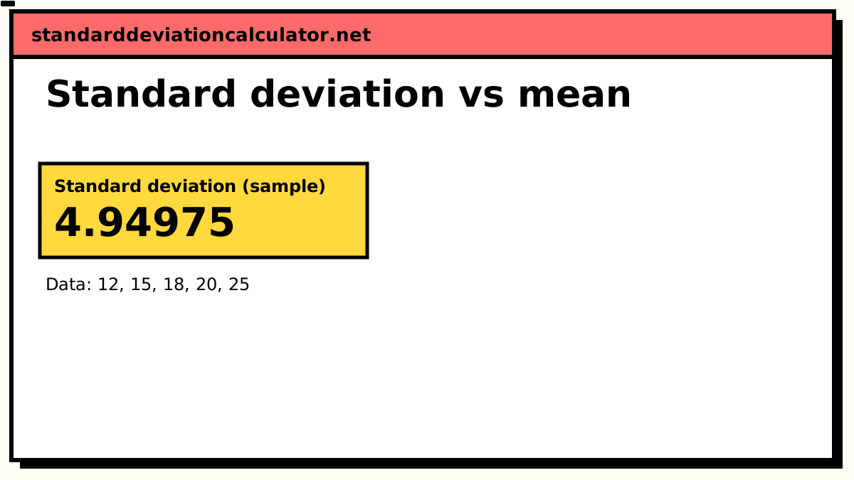
Standard deviation (sample)
4.94975
4.95
Your values typically sit about 4.95 above or below their mean of 18, in the same units as your data. 3 of 5 values (60%) fall between 13.05 and 22.95, within one standard deviation of the mean; for normally distributed data about 68% would.
Population SD (σ): 4.42719, if these values are the whole group.
- Count (n)
- 5
- Mean (x̄)
- 18
- Variance (s²)
- 24.5
- Standard error
- 2.21359
- Minimum
- 12
- Q1 (25%)
- 15
- Median
- 18
- Q3 (75%)
- 20
- Maximum
- 25
- Range
- 13
More statistics (5)
- Relative SD (%RSD)
- 27.4986%
- Coefficient of variation
- 0.274986
- Sum (Σx)
- 90
- Sum of squares, Σ(x − x̄)²
- 98
- IQR (Q3 − Q1)
- 5
Data distribution
Shaded bands mark ±1, ±2 and ±3 SD from the mean. 3 of 5 values (60%) fall within ±1 SD.
Chart as text
Mean 18, sample standard deviation s = 4.94975, from 5 values between 12 and 25.
- Within ±1 SD (13.05 to 22.95): 3 of 5 values (60%). About 68% for normal data.
- Within ±2 SD: 5 (100%). About 95% for normal data.
- Within ±3 SD: 5 (100%). About 99.7% for normal data.
Show the working, step by step
Reporting mean ± SD, and when it should be mean ± SE
The conventional way to give both is "mean ± SD": 18.0 ± 4.9 °C (n = 5). Written that way it describes the data. It says how much individual days varied, and for roughly bell-shaped data it lets a reader apply the 68–95–99.7 rule in their head.
"Mean ± SE" describes something else: how precisely the mean has been pinned down. The standard error is the SD divided by √n, so for the temperatures it is 4.95 ÷ √5 = 2.21 °C. The same data can therefore be written as 18.0 ± 4.9 or 18.0 ± 2.2, and a reader who does not know which was used will misread the spread by more than a factor of two. With n = 100 the gap becomes a factor of ten. Use the SD when describing a sample, the SE (or a confidence interval) when comparing means, and say which one it is every time.
The coefficient of variation: SD as a fraction of the mean
Divide the standard deviation by the mean and you get the coefficient of variation, usually given as a percentage:
CV = s / x̄ × 100% CV = 4.95 / 18 × 100% = 27.5%
The CV is the one place the two numbers are combined into a single figure. It is unit-free, so it lets you compare spread across data with very different means: routes A and B above have the same SD but CVs of 16.9% and 9.9%, because 4.74 minutes matters more on a 28-minute trip than on a 48-minute one. The coefficient of variation calculator works it out from raw data. It only makes sense for values measured from a true zero, as the next section shows.
Shifting and scaling: how each one responds
Transforming the data changes the mean and the SD in different ways, and the difference is a good test of what each one measures. Starting from the temperatures (mean 18, SD 4.95):
| Transformation | New values | Mean | SD | CV |
|---|---|---|---|---|
| None | 12, 15, 18, 20, 25 | 18 | 4.95 | 27.5% |
| Add 10 | 22, 25, 28, 30, 35 | 28 | 4.95 | 17.7% |
| Multiply by 3 | 36, 45, 54, 60, 75 | 54 | 14.85 | 27.5% |
| °C to °F (× 1.8 + 32) | 53.6, 59, 64.4, 68, 77 | 64.4 | 8.91 | 13.8% |
The general rule, for y = a·x + b:
mean(y) = a · mean(x) + b SD(y) = |a| · SD(x)
Adding a constant moves the mean and leaves the SD alone, because every value moves the same distance and no value gets closer to or further from the others. Multiplying scales both, and the SD by the absolute value of the multiplier, since a spread cannot be negative. The Fahrenheit row checks out: 1.8 × 18 + 32 = 64.4 and 1.8 × 4.95 = 8.91.
The CV column is the warning. Scaling leaves it unchanged, but shifting does not, so the same five days have a CV of 27.5% in Celsius and 13.8% in Fahrenheit. Neither is meaningful, because 0 °C and 0 °F are arbitrary points. Keep the CV for lengths, weights, times, counts and money.
What one outlier does to each
Suppose the sensor glitched on the last day and logged 60 instead of 25. The data is now
12, 15, 18, 20, 60.
| Statistic | Original | With 60 |
|---|---|---|
| Mean | 18 | 25 |
| Standard deviation | 4.95 | 19.80 |
| Median | 18 | 18 |
The mean moved 7 degrees; the SD quadrupled. The SD reacts harder because the outlier's deviation is squared: 60 sits 35 from the new mean, and its 35² = 1225 is 78% of the new sum of squares, 1568. The median did not move, and neither does the interquartile range (15 to 20 with the inclusive quartile method, in both cases). When the data has genuine extreme values or a long tail, report the median and IQR alongside, or instead of, the mean and SD. The outlier calculator flags suspect points before you commit to either.
Common mistakes
"The standard deviation can't be bigger than the mean." It can. Take the number of
prescriptions filled by seven patients in a year: 0, 0, 1, 1, 2, 3, 14. The mean
is 3 and the sample SD is 4.97. Nothing is wrong with the arithmetic. For data that cannot
go below zero, an SD above the mean does tell you something, though: the mean minus one SD is
−1.97, a value that cannot occur, so the data cannot be symmetric around its mean. It has a
long right tail, here a single heavy user, and the median of 1 describes a typical patient
better than the mean of 3. For data that can be negative, the comparison means nothing. A
fund's daily returns might average 0.05% with an SD of 1.2%, and the mean could as easily be
zero.
Writing mean ± 2 SD as a range for skewed data. With the prescription counts that range is 3 ± 9.93, running from −6.93 to 12.93. The lower end is impossible and the upper end excludes the one real extreme. The ± form assumes rough symmetry.
Comparing SDs across groups with very different means. An SD of 5 kg is large for newborns and small for adult cattle. Use the CV, or compare each SD with its own mean.
Reporting ± without saying whether it is SD or SE. As shown above, the two differ by a factor of √n, and a caption that says only "mean ± error" leaves the reader guessing.
Treating a low SD as a good result. The SD describes variation; it does not judge it. Whether variation is a problem depends on the mean and on what the data is for, which is the theme of the use cases page.
Related calculators
-
Mean and standard deviation calculator
Both numbers from one list of values, with the working shown.
-
Coefficient of variation calculator
The SD divided by the mean, as a percentage.
-
Standard deviation vs variance
The other comparison: the SD and its square.
-
Standard error calculator
SD ÷ √n, for when the question is the precision of the mean.
Common questions
What is the difference between the mean and the standard deviation?
The mean is the centre of the data: the sum of the values divided by how many there are. The standard deviation is the spread: the typical distance of a value from that mean. They answer different questions, so neither can be worked out from the other and a dataset is only summarised properly when you give both.
Can the standard deviation be larger than the mean?
Yes. The data 0, 0, 1, 1, 2, 3, 14 has a mean of 3 and a sample standard deviation of 4.97. For data that cannot go below zero, an SD larger than the mean is a sign of strong right skew. For data that can be negative, such as daily returns or temperature changes, it is ordinary and tells you nothing about shape.
Should I report mean ± SD or mean ± SE?
Use mean ± SD when you are describing how the individual values vary, which is the usual case in a table of sample characteristics. Use mean ± SE, or better a confidence interval, when the point is how precisely the mean itself has been estimated. Always label which one you used and give n, because SE = SD ÷ √n and the two look very different.
What happens to the mean and standard deviation if I add a constant to every value?
The mean goes up by that constant and the standard deviation does not change at all. Adding 10 to the values 12, 15, 18, 20, 25 moves the mean from 18 to 28, while the SD stays at 4.95. Every value moves by the same amount, so the distances between them, and from the mean, are unchanged.
Is a standard deviation that is half the mean high?
That ratio is the coefficient of variation, here 50%. Whether 50% is high depends on the field: it would be alarming for repeat measurements of a lab standard, where a few percent is typical, and unremarkable for household incomes or insurance claims. Compare it with the CV of similar data rather than with a fixed cut-off.