Sum of squares calculator
Enter your data to get the sum of squared deviations from the mean, Σ(x − x̄)². The result is shown both by the definition and by the Σx² − (Σx)²/n shortcut, along with the variance and standard deviation that follow from it, with the working laid out in full. In ANOVA and regression the same total is called SST and splits into SSR and SSE, covered below.
Separate numbers with commas, spaces or new lines, or paste a spreadsheet column.
Decimals and negatives are fine; write 10:3 for a value that occurs 3 times.
Your results will appear here: the result first, then the rest of the summary and a chart.
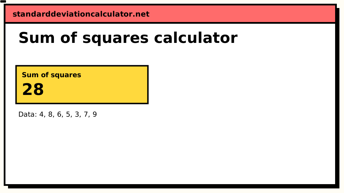
Sum of squared deviations
28
Data distribution
Shaded bands mark ±1, ±2 and ±3 SD from the mean. 5 of 7 values (71%) fall within ±1 SD.
Chart as text
Mean 6, sample standard deviation s = 2.16025, from 7 values between 3 and 9.
- Within ±1 SD (3.84 to 8.16): 5 of 7 values (71%). About 68% for normal data.
- Within ±2 SD: 7 (100%). About 95% for normal data.
- Within ±3 SD: 7 (100%). About 99.7% for normal data.
Show the working, step by step
The sum of squares formula
SS = Σ(x − x̄)²
Take each value, subtract the mean, square the difference, and add the squares together. The result is the sum of squares (more precisely the sum of squared deviations, since it is the deviations from the mean that are squared, not the values themselves). It is the total amount of variation in the data, before any averaging has taken place.
Almost every measure of spread in statistics starts here. The variance is this number divided by a count; the standard deviation is the square root of that; ANOVA and regression are accounts of how this number splits into parts. Understanding the sum of squares makes the rest of the subject considerably less mysterious.
Sum of squares: a worked example
Data: 4, 8, 6, 5, 3, 7, 9. The sum is 42 and n = 7, so the mean is
x̄ = 42 ÷ 7 = 6.
| x | x − x̄ | (x − x̄)² |
|---|---|---|
| 4 | −2 | 4 |
| 8 | 2 | 4 |
| 6 | 0 | 0 |
| 5 | −1 | 1 |
| 3 | −3 | 9 |
| 7 | 1 | 1 |
| 9 | 3 | 9 |
| Σ | 0 | 28 |
The sum of squares is 28. The middle column adds to zero, as it always does: the mean is by definition the point about which positive and negative deviations balance. That is the reason the deviations have to be squared before they are summed: added raw, they cancel to nothing whatever the data.
The computational shortcut
Expanding the square and simplifying gives a second form that avoids computing every deviation:
SS = Σx² − (Σx)² / n
For the example, Σx² = 16 + 64 + 36 + 25 + 9 + 49 + 81 = 280, and (Σx)²/n = 42² ÷ 7 = 1764 ÷ 7 = 252. So SS = 280 − 252 = 28, the same answer. The calculator above reports all three quantities so you can check either route.
The shortcut was invented for hand and desk-calculator arithmetic, where it saves a pass through the data, and textbooks still teach it for that reason. It is not what this site uses internally. Σx² and (Σx)²/n are both large numbers, and when the data has a big mean and a small spread they are nearly equal large numbers. Subtracting them throws away most of the significant digits, a failure known as catastrophic cancellation. On the three values 1000000.1, 1000000.2 and 1000000.3, whose sum of squares is exactly 0.02, the shortcut in double-precision arithmetic returns about 0.0195, and cruder implementations return zero or a small negative number, which is impossible. The calculator accumulates the squared deviations directly with Welford's method instead; the methodology page has the details.
From sum of squares to variance and standard deviation
The sum of squares is the numerator of the variance. Dividing it by a count turns a total into an average squared deviation:
Sample: s² = SS / (n − 1) Population: σ² = SS / n
For the example, SS = 28 divided by n − 1 = 6 gives a sample variance of 4.6667, and divided by n = 7 gives a population variance of 4. Which divisor applies depends on whether your seven numbers are the whole group you care about or a sample standing in for a larger one; the sample versus population guide sets out the reasoning, and the variance calculator makes the same computation with the variance as the headline figure.
The standard deviation is the square root of the variance: √4.6667 = 2.1602 for the sample and √4 = 2 for the population. So the full chain is sum of squares → divide by a count → take the square root, which is exactly the full standard deviation formula written out in steps. Each step is simple; the sum of squares is where the real work happens.
Total, between and within: sums of squares in ANOVA and regression
Once data is organised into groups, the single sum of squares splits into pieces, and the split is the whole idea behind analysis of variance. Three quantities appear in every ANOVA table:
- SST, the total sum of squares: every value's squared deviation from the grand mean of all the data.
- SSB, the between-groups sum of squares (also called treatment or model): each group's squared distance from the grand mean, weighted by its size.
- SSW, the within-groups sum of squares (also called SSE, the error sum of squares): each value's squared deviation from its own group's mean.
SST = SSB + SSW
The identity is exact, not approximate. Take two groups, 4, 6, 5 and
8, 10, 9. The grand mean is 7 and the total sum of squares is 28. The group
means are 5 and 9, each two units from the grand mean, so SSB = 3(−2)² + 3(2)² = 24. Within
each group the deviations are −1, 1, 0, so SSW = 2 + 2 = 4. And 24 + 4 = 28. The F statistic
is a ratio built from SSB and SSW, each divided by its degrees of freedom; the
ANOVA calculator produces the full table.
Regression uses the same decomposition with different labels. SST is again the total variation in y; SSR, the regression sum of squares, is the part the fitted line accounts for; SSE, the residual or error sum of squares, is what remains. The familiar R² is simply SSR / SST, the fraction of the total sum of squares the model explains. The linear regression calculator reports all three; the residual calculator lists each residual that goes into SSE, and the R² calculator works from SSR and SST directly.
Why square the deviations rather than take absolute values?
Squaring is not the only way to stop the deviations cancelling. Taking absolute values works too, and the result (the mean absolute deviation) is easier to explain. Squares won for three reasons. The squared deviation is smooth and differentiable, which is what makes least-squares problems solvable with calculus: the mean is the value that minimises the sum of squares, and the regression line is the line that does. Sums of squares add across independent sources of variation, which is what allows SST to be partitioned at all; absolute deviations do not. And for normally distributed data, the estimator built from squares is the most efficient one available.
The cost is sensitivity to outliers. A deviation of 10 contributes 100 to the sum of squares, while ten deviations of 1 contribute 10 between them, so a single distant value can dominate the total. That is a property to keep in mind, not a reason to abandon squares.
Units
Because every term is a squared deviation, the sum of squares is measured in the square of the data's units: kilograms squared, seconds squared, dollars squared. That is also why the variance is awkward to report and the standard deviation is preferred for description: the square root returns the answer to the units the data was measured in. The sum of squares itself is rarely quoted as a final result. It is an intermediate quantity, and the reason to compute it is what you do with it next.
Related calculators
-
Variance calculator
The sum of squares divided by n − 1 or n, with sample and population options.
-
Standard deviation calculator
The square root of the variance, back in the data’s own units.
-
ANOVA calculator
Total, between and within sums of squares for three or more groups.
-
Root mean square
The square root of the mean of the raw squares, Σx²/n.
Common questions
What is the sum of squares formula?
The definitional form is SS = Σ(x − x̄)²: subtract the mean from every value,
square each difference, and add the squares up. The algebraically equivalent shortcut is
SS = Σx² − (Σx)²/n, which needs only the sum of the values and the sum of their
squares.
Both give the same answer in exact arithmetic. This calculator shows both, but computes the result from the deviations, because the shortcut loses precision on data with a large mean.
What is the difference between the sum of squares and the variance?
The variance is the sum of squares divided by a count: by n − 1 for a sample, by n for a population. The sum of squares is the raw total of squared deviations before that division, so it grows as you add more data, whereas the variance settles towards a fixed value.
The variance calculator makes the same computation with the variance as the headline figure.
Can the sum of squares be negative?
No. Every term is a squared number, so the total is zero or positive. It is exactly zero only when every value equals the mean, that is, when all the values are identical.
If a spreadsheet formula built from the shortcut hands you a small negative number, it is floating-point cancellation, not a real result. See the methodology page for the example that breaks it.
What are SST, SSB and SSW (or SSE)?
They are the three sums of squares in an analysis of variance. SST, the total sum of squares, measures all the variation around the grand mean. SSB (between groups, also called the treatment or model sum of squares) measures how far the group means sit from the grand mean. SSW (within groups, also called SSE, the error sum of squares) measures scatter inside each group around its own mean. They always satisfy SST = SSB + SSW.
In regression the same split is written SST = SSR + SSE, with SSR the part explained by the fitted line.
Why is the sum of squares written with a capital S?
By convention, SS with a subscript names a sum of squares in a table: SStotal, SSbetween, SSwithin, SSxx, SSxy. A lower-case s² is a variance. The two are related by division: s² = SS / (n − 1).
How do I find the sum of squares in Excel?
=DEVSQ(A1:A20) returns Σ(x − x̄)² directly. =SUMSQ(A1:A20) is
different: it returns the raw Σx² without subtracting the mean, which is only the first
term of the shortcut formula. Confusing the two is the most common spreadsheet error with
this statistic.