Variance formula
Variance measures spread as the average squared distance from the mean. There are two everyday formulas, one for a sample and one for a whole population, plus versions for random variables, standard distributions and frequency tables. Each is below with a worked number, and the calculator applies them to your own data.
The two variance formulas
Sample variance: your numbers are a subset of a larger group.
s² = Σ(x − x̄)² / (n − 1)
Population variance: your numbers are the whole group.
σ² = Σ(x − μ)² / N
Both do the same four things: find the mean, subtract it from every value, square each
difference, and add the squares up. The only difference is the divisor, n − 1 for a sample
and N for a population. Coursework and most real data are samples, so when in doubt use
n − 1. In a spreadsheet the two are =VAR.S(A1:A100) and
=VAR.P(A1:A100).
Separate numbers with commas, spaces or new lines, or paste a spreadsheet column.
Decimals and negatives are fine; write 10:3 for a value that occurs 3 times.
Your results will appear here: the standard deviation first, then the rest of the summary and a chart.
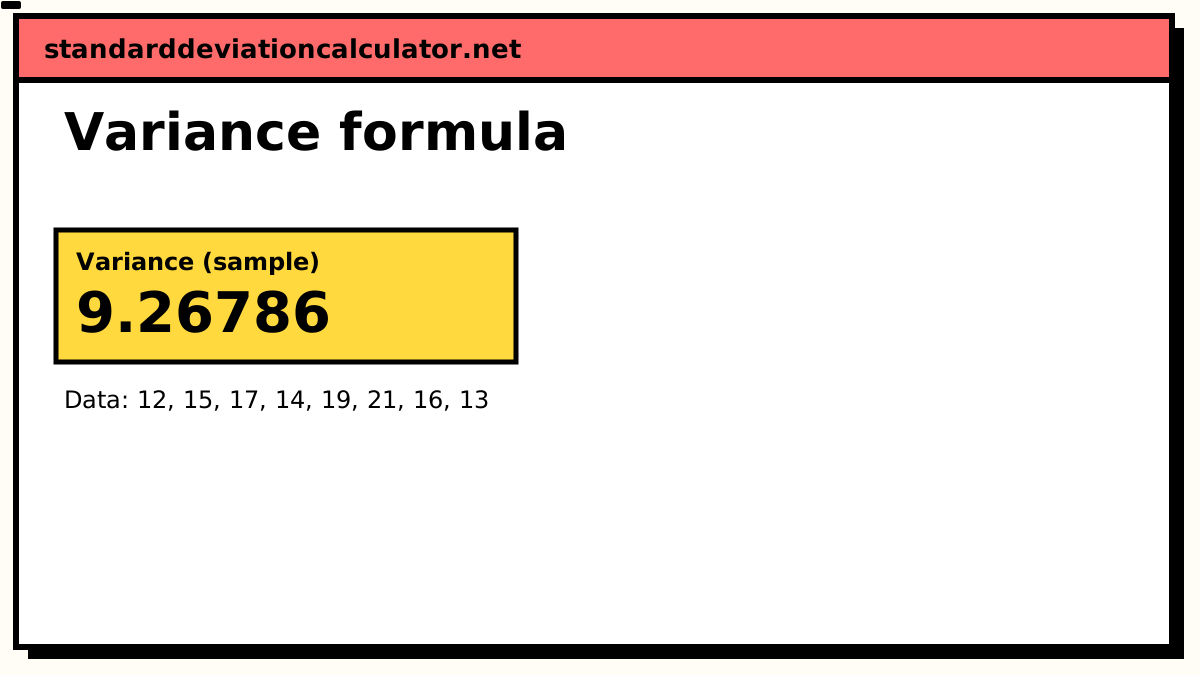
Variance (sample)
9.26786
9.27
The variance is in squared units, so it is hard to read on its own. Its square root is the standard deviation, 3.044: your values typically sit about that far above or below their mean of 15.88.
Population variance (σ²): 8.10938, if these values are the whole group.
- Count (n)
- 8
- Mean (x̄)
- 15.875
- Standard deviation (s)
- 3.04432
- Standard error
- 1.07633
- Minimum
- 12
- Q1 (25%)
- 13.75
- Median
- 15.5
- Q3 (75%)
- 17.5
- Maximum
- 21
- Range
- 9
More statistics (5)
- Relative SD (%RSD)
- 19.1768%
- Coefficient of variation
- 0.191768
- Sum (Σx)
- 127
- Sum of squares, Σ(x − x̄)²
- 64.875
- IQR (Q3 − Q1)
- 3.75
Data distribution
Shaded bands mark ±1, ±2 and ±3 SD from the mean. 5 of 8 values (63%) fall within ±1 SD.
Chart as text
Mean 15.875, sample standard deviation s = 3.04432, from 8 values between 12 and 21.
- Within ±1 SD (12.83 to 18.92): 5 of 8 values (63%). About 68% for normal data.
- Within ±2 SD: 8 (100%). About 95% for normal data.
- Within ±3 SD: 8 (100%). About 99.7% for normal data.
Show the working, step by step
Every symbol in the formula
| Symbol | Read as | Meaning |
|---|---|---|
| x or xᵢ | x, or "x sub i" | Each value in the data, taken in turn. |
| x̄ | x-bar | The sample mean. |
| μ | mu | The population mean. |
| n / N | n | The number of values: n for a sample, N for a population. |
| Σ | capital sigma | "Add up all of these." |
| s² / σ² | s squared, sigma squared | The sample and population variance. |
The symbols in the standard deviation formula are the same ones, with one square root added.
Variance formula example, step by step
Data: 3, 5, 7, 7, 8.
- Sum = 30, count n = 5, so the mean is 6.
- Deviations from the mean: −3, −1, 1, 1, 2.
- Squared: 9, 1, 1, 1, 4. Their sum, Σ(x − x̄)², is 16.
-
As a sample: 16 ÷ (5 − 1) = s² = 4.
As a population: 16 ÷ 5 = σ² = 3.2.
Paste the five values into the calculator above to check them, and switch between sample and population to see only the divisor change. The square roots, 2 and about 1.789, are the matching standard deviations.
Why n − 1 for a sample
The sample mean is calculated from the very values whose spread you are measuring, so it sits closer to them than the true population mean does. Squared distances around it are therefore too small on average, and dividing by n − 1 instead of n corrects that bias exactly. The effect is large for small samples (a quarter more variance at n = 5) and negligible for large ones. Sample vs population works through the reasoning in full.
The computational (shortcut) formula
s² = [ Σx² − (Σx)² / n ] / (n − 1)
It avoids computing each deviation. On the example data, Σx² = 196 and (Σx)²/n = 900/5 = 180, so s² = (196 − 180) / 4 = 4, the same answer. It is handy by hand but fragile on a computer: when the values are large and close together the subtraction loses most of its significant digits, which is why this site uses Welford's algorithm instead.
Variance of a random variable
For a random variable X with mean μ = E[X]:
Var(X) = E[(X − μ)²] = E[X²] − (E[X])²
- Discrete:
Var(X) = Σ (x − μ)² · p(x), summed over every value x. - Continuous:
Var(X) = ∫ (x − μ)² f(x) dx, integrated over the whole range.
Example, one roll of a fair die: E[X] = 3.5 and E[X²] = (1 + 4 + 9 + 16 + 25 + 36) / 6 = 91/6, so Var(X) = 91/6 − 3.5² = 35/12 ≈ 2.917. The expected value calculator does this for any probability table, and the standard deviation of a random variable takes the square root.
Variance of common distributions
| Distribution | Variance | Calculator |
|---|---|---|
| Binomial (n trials, success probability p) | np(1 − p) | Binomial |
| Poisson (rate λ) | λ | Poisson |
| Geometric (trials to first success, p) | (1 − p) / p² | Geometric |
| Continuous uniform on [a, b] | (b − a)² / 12 | Uniform |
| Discrete uniform on 1, 2, …, k | (k² − 1) / 12 | Dice average |
| Exponential (rate λ) | 1 / λ² | Exponential |
| Normal (mean μ, SD σ) | σ² | Normal |
The die example fits the discrete uniform row: k = 6 gives (36 − 1) / 12 = 35/12.
Variance for grouped and frequency data
When each value x occurs f times, weight every squared deviation by its frequency:
s² = Σf(x − x̄)² / (Σf − 1) where x̄ = Σfx / Σf
Example: the value 1 occurs 2 times, 2 occurs 3 times and 3 occurs 5 times. Then Σf = 10, Σfx = 23 and x̄ = 2.3. The weighted squared deviations are 2 × 1.69 + 3 × 0.09 + 5 × 0.49 = 6.1, so s² = 6.1 / 9 ≈ 0.678 (or σ² = 6.1 / 10 = 0.61 for a population). For class intervals, use each class midpoint as x; the result is then an approximation. The grouped-data calculator and the frequency table calculator show every column.
Variance of a sum or linear combination
Var(aX + bY) = a²Var(X) + b²Var(Y) + 2ab·Cov(X, Y)
Constants come out squared, and adding a constant does not change the variance at all: Var(X + c) = Var(X). When X and Y are independent their covariance is zero, so variances simply add, which is the main reason statistics works with variances rather than standard deviations. The covariance calculator gives Cov(X, Y) from paired data, and the portfolio standard deviation calculator applies this formula to two assets.
From variance to standard deviation
The standard deviation is the square root of the variance, s = √s², which puts the
spread back into the data's own units: a variance of 16 cm² is a standard deviation of 4 cm.
The standard deviation formula is therefore this
page's formula with one more step, and
standard deviation vs variance covers when to
report which.
Copy the formulas
Plain text, for Word, Google Docs or email:
s² = Σ(x − x̄)² / (n − 1)σ² = Σ(x − μ)² / NVar(X) = E[X²] − (E[X])²
LaTeX:
s^2 = \frac{\sum (x_i - \bar{x})^2}{n-1}\sigma^2 = \frac{\sum (x_i - \mu)^2}{N}\operatorname{Var}(X) = E[X^2] - (E[X])^2
In Google Docs choose Insert → Equation and type the LaTeX commands followed by a space; in Word press Alt+= and paste the LaTeX line with LaTeX selected in the Equation ribbon.
Related calculators
-
Variance calculator
Apply the formula to your own numbers, sample or population.
-
Standard deviation formula
The same formula with the square root taken, term by term.
-
SD vs variance
Which of the two to report, and why both exist.
-
Expected value calculator
E[X], E[X²] and the variance of a probability distribution.
-
Grouped data
Variance and SD from class intervals and frequencies.
-
The symbols explained
What xᵢ, x̄, n, Σ and s mean, with one worked example.
Common questions
What is the formula for variance?
For a sample: s² = Σ(x − x̄)² / (n − 1). For a population:
σ² = Σ(x − μ)² / N. Both add up the squared distances of the values from
their mean; the sample version divides by one less than the count.
Why does the sample variance divide by n − 1?
Because the sample mean x̄ is computed from the same values, so the values sit closer to x̄ than to the true population mean. Dividing by n would understate the population variance on average; dividing by n − 1 removes that bias exactly. This is Bessel's correction.
What is xᵢ in the variance formula?
xᵢ ("x sub i") is the i-th value in the data: x₁ is the first, x₂ the second, up to xₙ. Writing Σ(xᵢ − x̄)² means "for every value, subtract the mean, square the result, then add them all up". Many books drop the subscript and write Σ(x − x̄)², which means the same thing.
How do you find the variance from the expected value?
Use Var(X) = E[X²] − (E[X])²: the mean of the squares minus the square of the
mean. For a fair six-sided die, E[X] = 3.5 and E[X²] = 91/6, so
Var(X) = 91/6 − 12.25 = 35/12 ≈ 2.917.
What is the variance of a binomial distribution?
Var(X) = np(1 − p), where n is the number of trials and p the probability of
success on each. Ten fair coin flips have a variance of 10 × 0.5 × 0.5 = 2.5 heads².
How do you get the standard deviation from the variance?
Take the square root: s = √s² and σ = √σ². A variance of 4
is a standard deviation of 2. Going the other way, square the standard deviation.