Exponential distribution calculator
Enter the rate λ (or the mean time between events), then a time x. The calculator gives the probability of waiting at most x, at least x or between two times, or the time by which a given share of waits are over.
Greater than 0, e.g. 0.5 arrivals per minute.
Greater than 0, e.g. 2 minutes between arrivals.
Between 0 and 1, e.g. 0.95 or 95%.
The curve is the probability density; the shaded area is the probability asked for.
| P(X ≤ x) | 0.01 | 0.05 | 0.25 | 0.5 | 0.75 | 0.95 | 0.99 |
|---|---|---|---|---|---|---|---|
| x | 0.020101 | 0.10259 | 0.57536 | 1.3863 | 2.7726 | 5.9915 | 9.2103 |
Show the working, step by step
Put x into the cumulative distribution function F(x) = P(X ≤ x):
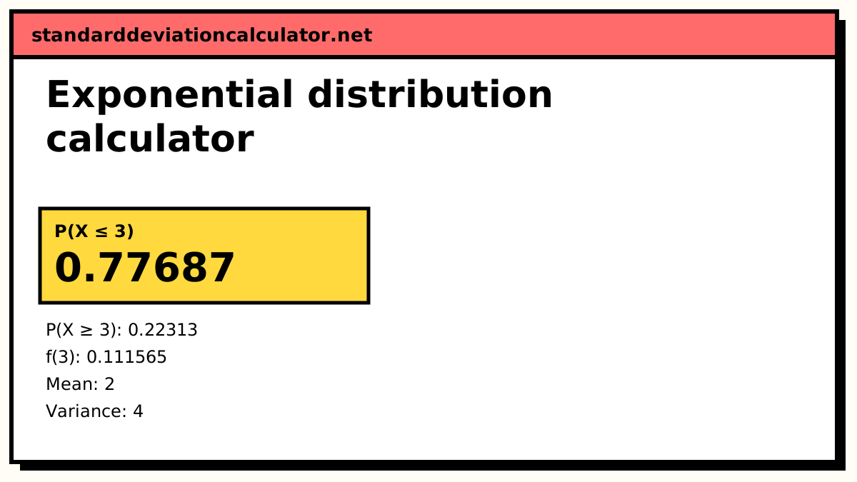
F(x) = 1 − e−λx F(3) = 1 − e−0.5 × 3 = 1 − e−1.5 = 1 − 0.22313 = 0.77687
The formulas
f(x) = λe−λx, x ≥ 0 F(x) = P(X ≤ x) = 1 − e−λx P(X ≥ x) = e−λx xp = −ln(1 − p) / λ
mean = 1/λ variance = 1/λ² SD = 1/λ median = ln 2 / λ mode = 0
Worked example
Customers reach a counter at an average rate of λ = 0.5 per minute, so the mean gap between them is 2 minutes. What is the probability that the next customer arrives within 3 minutes?
P(X ≤ 3) = 1 − e−0.5 × 3 = 1 − e−1.5 = 1 − 0.22313 = 0.77687
So there is a 77.7% chance of an arrival within 3 minutes and a 22.3% chance the gap is longer. The density at x = 3 is 0.5 × 0.22313 = 0.111565 per minute.
For an interval, subtract two CDF values. The chance the gap is between 1 and 4 minutes is (1 − e−2) − (1 − e−0.5) = 0.864665 − 0.393469 = 0.471195.
Going the other way, the 90th percentile is −ln(0.1) / 0.5 = 4.60517 minutes: nine gaps in ten are shorter than that. The median is ln 2 / 0.5 = 1.38629 minutes, the mean and standard deviation are both 2 minutes, and the variance is 4.
Reading the result
The chart shows why most waits are short. The density is highest at 0 and falls by the same factor over every interval of equal length: each extra minute multiplies the survival probability by e−0.5 = 0.607. That constant ratio is the memoryless property, and it is also the assumption you should question. Arrivals at a shop that are bunched at lunchtime, or machines that wear out, are not exponential; the Weibull distribution relaxes the constant rate.
Common mistakes
- Entering the mean as the rate. λ is events per unit time; the mean is time per event. They are reciprocals.
- Mixing units. If λ is per hour, x must be in hours. Convert 3 minutes to 0.05 hours first.
- Using the Poisson formula for a waiting time. The Poisson answers “how many in an interval”; the exponential answers “how long until the next”.
- Assuming the mean is a typical value. With this much skew, 63.2% of waits are shorter than the mean, since F(1/λ) = 1 − e−1 = 0.632.
Common questions
What does the exponential distribution model?
The waiting time until the next event when events happen independently at a constant average rate: the time to the next customer, the next radioactive decay, or the next failure of a component that does not wear out. It is the continuous partner of the Poisson distribution, which counts how many of those events land in a fixed interval.
Rate or mean: which should I enter?
Either. They are reciprocals: a rate of λ = 0.5 arrivals per minute is the same as a mean wait of 1/λ = 2 minutes. Pick whichever your problem states and the calculator converts. Mixing them up is the most common exponential mistake: a mean of 2 entered as a rate gives P(X ≤ 3) = 0.9975 instead of 0.77687.
What is the memoryless property?
P(X > s + t | X > s) = P(X > t). Having already waited s minutes tells you nothing about the remaining wait. With λ = 0.5, the chance of waiting more than 3 more minutes is 0.22313 whether you have just arrived or have been waiting for ten minutes. The exponential is the only continuous distribution with this property.
Why is the median smaller than the mean?
The distribution is skewed right: most waits are short, but a few are very long and pull the mean up. The median is ln 2 / λ = 0.693/λ, about 69% of the mean. With a mean of 2 minutes, half of all waits are shorter than 1.386 minutes.
What is the standard deviation of an exponential distribution?
It equals the mean, 1/λ. The variance is 1/λ². So an exponential with a mean wait of 2 minutes has a standard deviation of 2 minutes as well, and a coefficient of variation of exactly 1.
Related calculators
-
Poisson distribution
Counts of events per interval at the same constant rate λ.
-
Weibull distribution
Generalises the exponential to failure rates that rise or fall with time.
-
Geometric distribution
The discrete version: trials until the first success.