Geometric distribution calculator
Enter the probability of success on each trial and pick whether X counts trials up to the first success or failures before it. The calculator gives P(X = k), P(X ≤ k), P(X ≥ k) or a range, with the working and a chart.
On each trial, between 0 and 1.
Between 0 and 1. Gives the smallest k with P(X ≤ k) ≥ p.
Each bar is P(X = k). Solid bars are the values included in the answer.
Probability table
| k | P(X = k) | P(X ≤ k) | P(X ≥ k) |
|---|---|---|---|
| 1 | 0.2 | 0.2 | 1 |
| 2 | 0.16 | 0.36 | 0.8 |
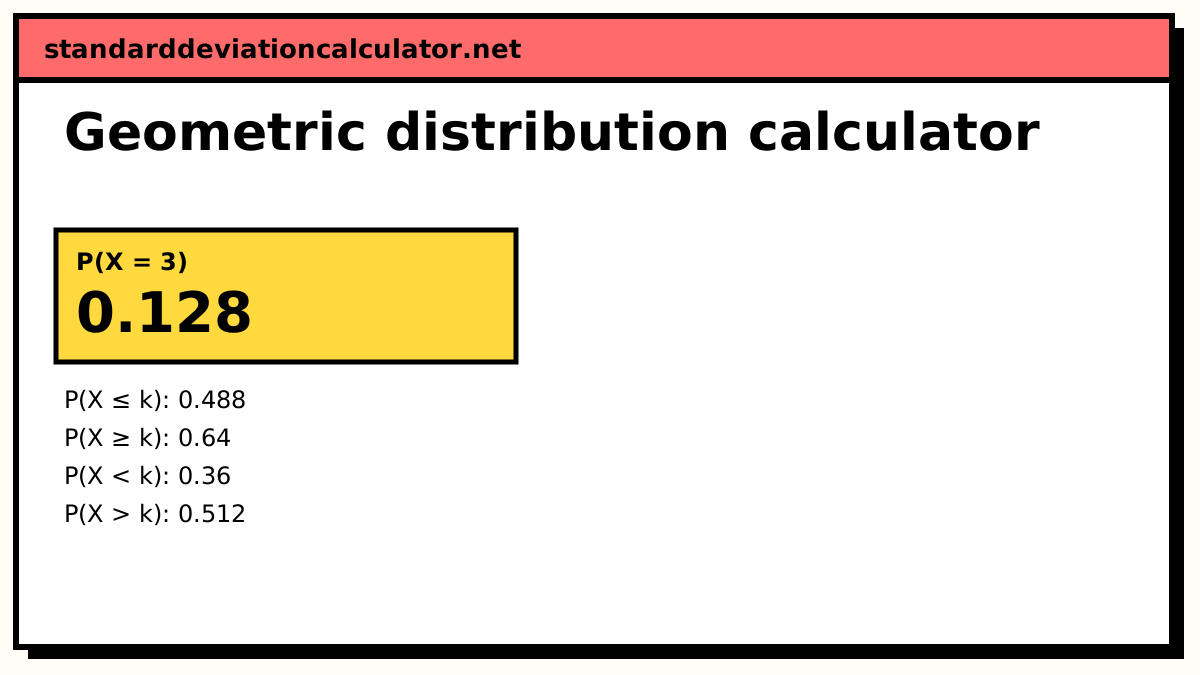
| 3 | 0.128 | 0.488 | 0.64 |
| 4 | 0.1024 | 0.5904 | 0.512 |
| 5 | 0.08192 | 0.67232 | 0.4096 |
| 6 | 0.065536 | 0.737856 | 0.32768 |
| 7 | 0.0524288 | 0.790285 | 0.262144 |
| 8 | 0.041943 | 0.832228 | 0.209715 |
| 9 | 0.0335544 | 0.865782 | 0.167772 |
| 10 | 0.0268435 | 0.892626 | 0.134218 |
| 11 | 0.0214748 | 0.914101 | 0.107374 |
| 12 | 0.0171799 | 0.931281 | 0.0858993 |
| 13 | 0.0137439 | 0.945024 | 0.0687195 |
| 14 | 0.0109951 | 0.95602 | 0.0549756 |
| 15 | 0.00879609 | 0.964816 | 0.0439805 |
| 16 | 0.00703687 | 0.971853 | 0.0351844 |
| 17 | 0.0056295 | 0.977482 | 0.0281475 |
| 18 | 0.0045036 | 0.981986 | 0.022518 |
| 19 | 0.00360288 | 0.985588 | 0.0180144 |
| 20 | 0.0028823 | 0.988471 | 0.0144115 |
| 21 | 0.00230584 | 0.990777 | 0.0115292 |
| 22 | 0.00184467 | 0.992621 | 0.00922337 |
| 23 | 0.00147574 | 0.994097 | 0.0073787 |
| 24 | 0.00118059 | 0.995278 | 0.00590296 |
| 25 | 0.000944473 | 0.996222 | 0.00472237 |
| 26 | 0.000755579 | 0.996978 | 0.00377789 |
| 27 | 0.000604463 | 0.997582 | 0.00302231 |
| 28 | 0.00048357 | 0.998066 | 0.00241785 |
| 29 | 0.000386856 | 0.998453 | 0.00193428 |
| 30 | 0.000309485 | 0.998762 | 0.00154743 |
| 31 | 0.000247588 | 0.99901 | 0.00123794 |
| 32 | 0.00019807 | 0.999208 | 0.000990352 |
| 33 | 0.000158456 | 0.999366 | 0.000792282 |
| 34 | 0.000126765 | 0.999493 | 0.000633825 |
| 35 | 0.000101412 | 0.999594 | 0.00050706 |
Show the working, step by step
The cumulative probability has a closed form, because “at most k” is the complement of “the first k all fail”:
P(X ≤ k) = 1 − (1 − p)k
Probability of exactly k:
P(X = k) = (1 − p)k−1 p P(X = 3) = 0.82 × 0.2 = 0.64 × 0.2 = 0.128
The formulas
X = number of trials up to and including the first success (k = 1, 2, 3, …):
P(X = k) = (1 − p)k−1 p P(X ≤ k) = 1 − (1 − p)k mean = 1/p variance = (1 − p)/p²
Y = number of failures before the first success (k = 0, 1, 2, …):
P(Y = k) = (1 − p)k p P(Y ≤ k) = 1 − (1 − p)k+1 mean = (1 − p)/p variance = (1 − p)/p²
Worked example
A salesperson closes 20% of calls, independently. What is the probability that the first sale comes on the third call?
P(X = 3) = 0.8² × 0.2 = 0.64 × 0.2 = 0.128
Two failures then a success: 12.8%. The chance of a sale within the first three calls is 1 − 0.8³ = 0.488, and the chance of needing three or more calls is P(X ≥ 3) = 0.8² = 0.64. On average the first sale takes 1/0.2 = 5 calls, with a standard deviation of √20 = 4.47214. The median is 4 calls, since P(X ≤ 3) = 0.488 falls just short of one half and P(X ≤ 4) = 0.5904 passes it. The mode is always 1: a success on the very first trial is the single most likely outcome.
In the failures convention the same event is “2 failures before the first sale”, so P(Y = 2) = 0.8² × 0.2 = 0.128, the same number with k shifted down by one. The mean becomes 0.8/0.2 = 4 failures.
Reading the result
The bars fall by the same factor, 1 − p, from each k to the next, so the chart always decays geometrically, which is where the name comes from. Solid bars mark the values included in the probability you asked for. Open the probability table for P(X = k), P(X ≤ k) and P(X ≥ k) at every value in the bulk of the distribution.
Common mistakes
- Mixing conventions. An answer that is off by one trial almost always comes from this.
- Using the binomial formula. The binomial fixes the number of trials; the geometric fixes the number of successes (one) and lets the trials vary.
- Adding the terms one by one for P(X ≤ k). The closed form 1 − (1 − p)k is exact and quicker.
- Forgetting independence. If each failure changes the next chance (learning, fatigue), the geometric does not apply.
Common questions
Which geometric distribution convention should I use?
Check what your textbook or software counts. Most introductory statistics courses and the TI-84 (geometpdf) count trials up to and including the first success, so X starts at 1. R's dgeom, SciPy's nbinom and many probability texts count failures before the first success, so X starts at 0. The two differ by exactly 1: Xtrials = Xfailures + 1.
What is the mean of a geometric distribution?
1/p trials, or (1 − p)/p failures. With p = 0.2 you need 5 trials on average, 4 of them failures. The variance is (1 − p)/p² = 20 in both conventions, because shifting by 1 does not change the spread.
How do I find the probability of success within k trials?
P(X ≤ k) = 1 − (1 − p)k. The only way not to have succeeded by trial k is to fail k times in a row. With p = 0.2 and k = 3, that is 1 − 0.8³ = 1 − 0.512 = 0.488.
Is the geometric distribution memoryless?
Yes, it is the only discrete distribution that is. After any number of failures, the chance of needing more than j further trials is still (1 − p)j. A slot machine that has not paid out for 50 spins is no more “due” than on the first spin, if the spins are independent.
Related calculators
-
Negative binomial distribution
Trials until the r-th success; the geometric is the case r = 1.
-
Binomial distribution
Successes in a fixed number of trials.
-
Exponential distribution
The continuous waiting-time version.