Beta distribution calculator
Enter the two shape parameters α and β, then a value of x between 0 and 1. The calculator gives the probability to the left, to the right or between two values, or finds x for a given percentile, and draws the density with the area shaded.
Greater than 0. Think of it as successes + 1.
Greater than 0. Think of it as failures + 1.
Between 0 and 1, e.g. 0.95 or 95%.
The curve is the probability density; the shaded area is the probability asked for.
| P(X ≤ x) | 0.01 | 0.05 | 0.25 | 0.5 | 0.75 | 0.95 | 0.99 |
|---|---|---|---|---|---|---|---|
| x | 0.026763 | 0.06285 | 0.16116 | 0.26445 | 0.38948 | 0.5818 | 0.70569 |
Show the working, step by step
The beta function scales the density so it integrates to 1:
B(α, β) = Γ(α)Γ(β) / Γ(α + β) = Γ(2)Γ(5) / Γ(7) = 0.0333333
Put x into the cumulative distribution function F(x) = P(X ≤ x):
F(x) = Ix(α, β) = (1 / B(α, β)) ∫₀ˣ tα−1(1 − t)β−1 dt F(0.3) = I0.3(2, 5) = 0.579825
The formulas
f(x) = xα−1(1 − x)β−1 / B(α, β), 0 ≤ x ≤ 1 B(α, β) = Γ(α)Γ(β) / Γ(α + β) F(x) = P(X ≤ x) = Ix(α, β)
mean = α / (α + β) variance = αβ / [(α + β)²(α + β + 1)] mode = (α − 1) / (α + β − 2), α, β > 1
B(α, β) is the beta function, which scales the curve so the total area is 1. Ix(α, β) is the regularised incomplete beta function: the share of that area lying to the left of x.
Worked example
The default is Beta(2, 5) and x = 0.3. Suppose it describes your belief about a click-through rate after seeing 1 click in 5 impressions with a flat prior. What is the chance the true rate is at most 30%?
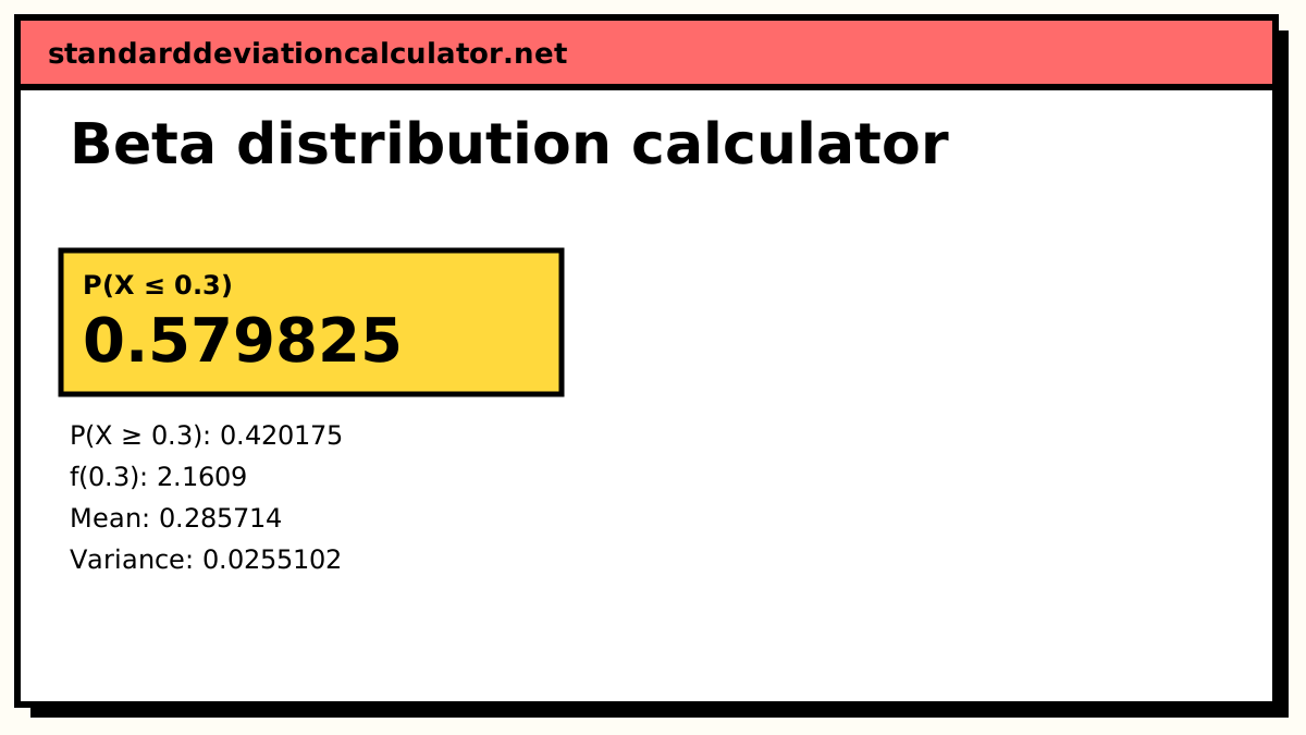
B(2, 5) = Γ(2)Γ(5) / Γ(7) = 1 × 24 / 720 = 1/30 = 0.0333333 f(0.3) = 30 × 0.3 × 0.7⁴ = 2.1609 P(X ≤ 0.3) = I0.3(2, 5) = 0.579825
Because α and β are whole numbers you can check this with a binomial tail: I0.3(2, 5) = P(Bin(6, 0.3) ≥ 2) = 1 − 0.7⁶ − 6 × 0.3 × 0.7⁵ = 1 − 0.117649 − 0.302526 = 0.579825. The right tail P(X ≥ 0.3) is 1 − 0.579825 = 0.420175.
The summary statistics are mean 2/7 = 0.285714, variance 10 / (49 × 8) = 0.0255102, standard deviation 0.159719, mode (2 − 1)/(7 − 2) = 0.2 and median 0.26445. The mode, median and mean appear in that order from left to right because the curve has a longer right tail.
Reading the result
P(X ≤ x) is the area under the density to the left of x, which is the shaded region on the chart. The density value f(x) is a height, not a probability, and can be larger than 1: here f(0.3) = 2.16. Only areas are probabilities.
The percentile table under the chart is often more useful than a single tail probability. For Beta(2, 5) the 5th and 95th percentiles are 0.06285 and 0.5818, so a 90% credible interval for the rate runs from about 6.3% to 58%. With so little data, that is wide, and it narrows as α + β grows.
Common mistakes
- Swapping α and β. Beta(5, 2) is the mirror image of Beta(2, 5), with its peak at 0.8 instead of 0.2.
- Treating f(x) as a probability. For a continuous variable P(X = x) is 0; the density only tells you where probability is concentrated.
- Entering counts directly as α and β when you meant a flat Beta(1, 1) prior plus data. The posterior after s successes and f failures is Beta(1 + s, 1 + f).
- Entering x outside 0 to 1. The distribution has no mass there, so the calculator returns 0 or 1.
Common questions
What is the beta distribution used for?
Modelling a quantity that must lie between 0 and 1: a proportion, a rate or a probability. Its best-known use is as the prior and posterior for an unknown success probability in Bayesian statistics. It also describes order statistics of uniform samples and task-completion fractions in project planning (PERT).
What do α and β mean?
Both are shape parameters. A handy reading is α − 1 successes and β − 1 failures: Beta(2, 5) looks like the likelihood after 1 success and 4 failures, so it peaks at 1/5 = 0.2. Larger α pushes the mass towards 1, larger β towards 0, and larger α + β makes the curve narrower.
How is the beta CDF calculated?
P(X ≤ x) is the regularised incomplete beta function Ix(α, β). It has no elementary closed form in general, so the calculator evaluates it with a continued fraction (Lentz's method), the same approach as Numerical Recipes. For whole-number α and β it equals a binomial tail: Ix(α, β) = P(Bin(α + β − 1, x) ≥ α).
What happens when α or β is below 1?
The density becomes infinite at that edge. With α < 1 the curve shoots up at 0; with β < 1 it shoots up at 1; with both below 1 you get a U shape, such as the arcsine distribution Beta(0.5, 0.5). Probabilities are still finite and the calculator handles them; the chart clips the spike so the rest of the curve stays visible.
How do I find the median or a percentile?
Choose “x from a probability” and enter the percentile as a proportion. The calculator solves Ix(α, β) = p by bisection. For Beta(2, 5) the median is 0.26445 and the 95th percentile is 0.581803.
Related calculators
-
Binomial distribution
The count of successes whose success rate the beta distribution describes.
-
Uniform distribution
Beta(1, 1) is the uniform distribution on 0 to 1.
-
Bayes' theorem
Update a probability with evidence; the beta is the standard prior for a rate.