Lognormal distribution calculator
Enter the lognormal parameters μ and σ (the mean and standard deviation of ln X), or the mean and SD of X itself. Then ask for the probability below, above or between values, or for a percentile.
Greater than 0.
Between 0 and 1, e.g. 0.95 or 95%.
The curve is the probability density; the shaded area is the probability asked for.
| P(X ≤ x) | 0.01 | 0.05 | 0.25 | 0.5 | 0.75 | 0.95 | 0.99 |
|---|---|---|---|---|---|---|---|
| x | 2.309 | 3.2465 | 5.2738 | 7.3891 | 10.353 | 16.818 | 23.646 |
Show the working, step by step
Put x into the cumulative distribution function F(x) = P(X ≤ x):
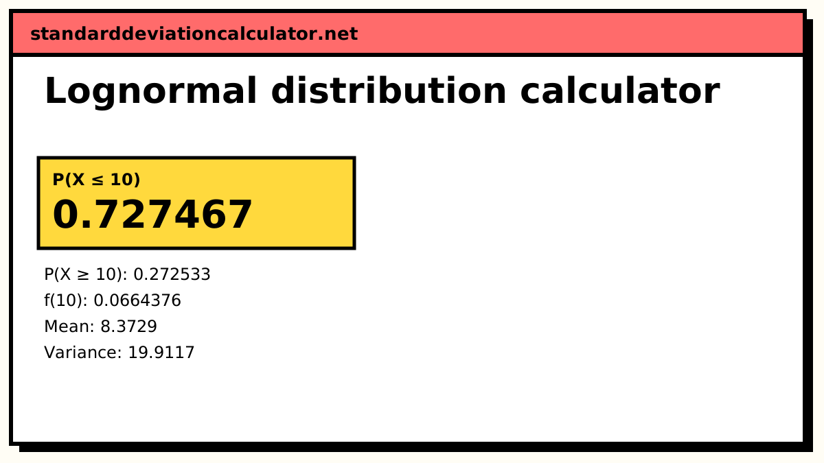
F(x) = Φ((ln x − μ) / σ) z = (ln 10 − 2) / 0.5 = (2.30259 − 2) / 0.5 = 0.60517 F(10) = Φ(0.60517) = 0.727467
The formulas
f(x) = 1 / (xσ√(2π)) · e−(ln x − μ)² / (2σ²), x > 0 F(x) = Φ((ln x − μ) / σ) xp = eμ + σ zp, zp = Φ⁻¹(p)
mean = eμ + σ²/2 median = eμ mode = eμ − σ² variance = (eσ² − 1) e2μ + σ²
Every lognormal probability is a normal probability in disguise: take the log of x, standardise it with μ and σ, and look up Φ.
Worked example
Repair times at a service desk are lognormal with μ = 2 and σ = 0.5 (log-hours). What share of repairs finish within 10 hours?
z = (ln 10 − 2) / 0.5 = (2.30259 − 2) / 0.5 = 0.60517 P(X ≤ 10) = Φ(0.60517) = 0.727467
About 72.7% of repairs take 10 hours or less, and 27.3% take longer. The typical repair (the median) takes e² = 7.389 hours, the average is e2.125 = 8.3729 hours, and the standard deviation is 4.46225 hours.
For a service-level target, ask for the 95th percentile instead: z0.95 = 1.64485, so x = e2 + 0.5 × 1.64485 = e2.82243 = 16.8176 hours. One repair in twenty takes longer than that.
When the lognormal fits
A quick check on real data: take the natural log of every value and look at the result. If the logs look roughly symmetric and bell-shaped, the lognormal is a reasonable model, and the mean and standard deviation of the logs are your estimates of μ and σ. A ratio of mean to median well above 1 in the raw data is another hint; for a lognormal it equals eσ²/2, which is 1.133 in the example above. If the data include zeros, the lognormal cannot fit them as they stand.
Reading the result
On the chart the peak sits well left of the mean and the right tail runs on for a long way. That shape is why reports of lognormal data should quote the median, or the geometric mean and geometric SD, rather than the arithmetic mean ± SD. Mean ± 2 SD here would be 8.37 ± 8.92, which runs below zero even though no repair can take negative time.
Common mistakes
- Entering the mean and SD of X as μ and σ. They are parameters of ln X; use the second input mode if you have the raw-scale figures.
- Using log base 10. The formulas use the natural log. If your μ and σ come from log10 data, multiply both by ln 10 = 2.302585.
- Assuming eμ is the mean. It is the median; the mean is larger by a factor of eσ²/2.
- Entering x ≤ 0. A lognormal variable is always positive, so P(X ≤ 0) = 0.
Common questions
What is a lognormal distribution?
A variable X is lognormal when its logarithm ln X is normally distributed. X is always positive and skewed to the right. It arises when many small effects multiply rather than add: incomes, city sizes, particle sizes, stock prices, repair times and the concentration of a pollutant are often close to lognormal.
Are μ and σ the mean and standard deviation of X?
No, and this is the usual source of wrong answers. μ and σ are the mean and standard deviation of ln X. With μ = 2 and σ = 0.5, the mean of X is e2.125 = 8.3729 and its SD is 4.46225. If your data give you the mean and SD of X itself, pick “Mean and SD of X” and the calculator converts them.
How do I convert the mean and SD of X into μ and σ?
σ² = ln(1 + SD²/mean²) and μ = ln(mean) − σ²/2. With a mean of 8.37 and SD of 4.46, σ² = ln(1 + 19.8916/70.0569) = 0.24993, so σ = 0.49993 and μ = ln 8.37 − 0.12496 = 1.99969, close to the μ = 2, σ = 0.5 of the default.
Why is the median e^μ?
Taking logs does not change the order of values, so the median of X is e raised to the median of ln X, which is μ. With μ = 2 the median is e² = 7.38906. The mean is larger (8.3729) because of the long right tail, and the mode is smaller: eμ − σ² = 5.7546.
What is the geometric standard deviation?
eσ, a multiplicative spread. With σ = 0.5 it is 1.64872, so about 68% of values lie between the median divided by 1.649 and the median times 1.649: from 4.48 to 12.18. Environmental and pharmacokinetic reports often quote the geometric mean (the median) and geometric SD.
Related calculators
-
Normal distribution
The distribution of ln X, which the lognormal is built from.
-
Geometric mean
The natural average for lognormal data: an estimate of e^μ.
-
Weibull distribution
Another skewed, positive model used for lifetimes and sizes.