SMp(x) distribution calculator
Enter the limits PXmin and Xmax, the peak position ML and the two powers p₁ and p₂. The calculator evaluates SMp(x), sets Max so the distribution is properly scaled, and gives probabilities, percentiles, the mean and the standard deviation.
0 or more. 1 gives a straight line.
0 or more.
Leave blank to have Max chosen so the probabilities add to 1.
Between 0 and 1. For a discrete variable, gives the smallest x with P(X ≤ x) ≥ p.
The curve is the probability density; the shaded area is the probability asked for.
| P(X ≤ x) | 0.01 | 0.05 | 0.25 | 0.5 | 0.75 | 0.95 | 0.99 |
|---|---|---|---|---|---|---|---|
| x | 1.1079 | 1.8945 | 3.2396 | 4.0851 | 5.0262 | 6.6738 | 7.7757 |
Show the working, step by step
Area under the curve with Max = 1 (each side integrates to width ÷ (power + 1)):
A = (ML − PXmin)/(p₁ + 1) + (Xmax − ML)/(p₂ + 1) = 4/3 + 6/4 = 2.83333
Choose Max so the total area is 1:
Max = 1 / A = 1 / 2.83333 = 0.352941
Put x into the cumulative distribution function F(x) = P(X ≤ x):
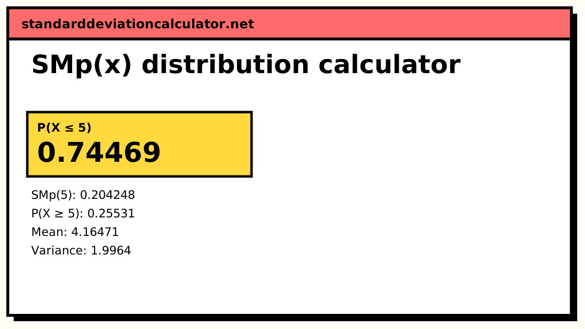
On the falling side, F(x) = 1 − (Xmax − ML)/(p₂ + 1) × [(Xmax − x)/(Xmax − ML)]p₂+1 ÷ A F(5) = 1 − 1.5 × 0.482253 ÷ 2.83333 = 0.74469
Height of the curve at x (the falling piece applies):
SMp(5) = [(10 − 5) / 6]3 × 0.352941 = 0.204248
The SMp(x) function
SMp(x) = 0, x < PXmin SMp(x) = [(x − PXmin)/(ML − PXmin)]p₁ × Max, PXmin ≤ x ≤ ML SMp(x) = [(Xmax − x)/(Xmax − ML)]p₂ × Max, ML ≤ x ≤ Xmax SMp(x) = 0, x > Xmax
PXmin and Xmax are the lower and upper limits of x, ML is where the function reaches its maximum, p₁ and p₂ are the powers of the rising and falling sides (both 0 or more), and Max is the peak height. For a continuous variable the area under the curve is
A = Max × [(ML − PXmin)/(p₁ + 1) + (Xmax − ML)/(p₂ + 1)]
and setting A = 1 fixes Max.
Worked example
The default is PXmin = 0, Xmax = 10, ML = 4, p₁ = 2 and p₂ = 3, a right-skewed curve. With Max left blank:
A (with Max = 1) = 4/3 + 6/4 = 2.83333 Max = 1 / 2.83333 = 0.352941 SMp(5) = [(10 − 5)/6]³ × 0.352941 = 0.578704 × 0.352941 = 0.204248
x = 5 is past the peak, so the falling side applies. The probability of a value at or below 5 subtracts the area to the right of 5 from 1:
P(X ≤ 5) = 1 − (6/4) × (5/6)⁴ ÷ 2.83333 = 1 − 1.5 × 0.482253 ÷ 2.83333 = 0.74469
So P(X ≥ 5) = 0.25531. The distribution has mean 4.16471, variance 1.9964, standard deviation 1.41294, median 4.08513 and mode ML = 4. The mean sits right of the mode because the falling side is longer.
Switch the variable to discrete and X takes only the whole numbers 0 to 10. The SMp values with Max = 1 add up to 2.91667, so Max = 1/2.91667 = 0.342857, and P(X = 4) = 1 × 0.342857 = 0.342857.
Reading the result
SMp(x) itself is a height. For a continuous variable it is a density, and probabilities are areas under it, shown shaded on the chart. For a discrete variable SMp(k) is the probability of k directly, as long as Max gives a total of 1. If you entered your own Max and see a warning, the total differs from 1 and the probabilities have been rescaled.
Common mistakes
- Putting ML outside the range. ML must lie between PXmin and Xmax.
- Expecting normal-like tails beyond the limits. SMp(x) is exactly 0 below PXmin and above Xmax.
- Reading the continuous SMp(x) value as a probability. It is a density height; only areas are probabilities.
- Choosing Max by eye. Leave it blank unless you are reproducing a published parameter set.
Common questions
What is the SMp(x) distribution?
A six-parameter probability function, SMp(x; PXmin, Xmax, ML, p₁, p₂, Max), proposed by Terman Frometa-Castillo (ITNG 2019, Springer). It is built from the triangular distribution: the curve rises from zero at PXmin to a peak of height Max at ML, then falls back to zero at Xmax. The powers p₁ and p₂ bend each side, so one formula can imitate normal, binomial, Poisson and skewed shapes, for either a continuous or a discrete variable.
How do I make SMp(x) look like a normal distribution?
Make it symmetric and give both sides the same power above 1: ML = (PXmin + Xmax)/2 and p₁ = p₂ > 1. The area is then 1 when Max = (p₁ + 1) / [2(ML − PXmin)], which is what the calculator picks if you leave Max blank. Unlike a true normal, the SMp curve reaches zero at PXmin and Xmax, so its tails are bounded.
What happens when p₁ = p₂ = 1?
Both sides are straight lines and SMp(x) is the triangular distribution with minimum PXmin, mode ML and maximum Xmax. Powers below 1 make the sides bulge outward (a fatter, flatter peak); powers above 1 make them sag inward (a sharper peak and thinner tails). A power of 0 makes that side flat at height Max.
Why is Max optional?
Max is the height of the peak, and for SMp(x) to be a probability distribution the total area (continuous) or total of the values (discrete) must be 1. There is exactly one Max that does that, so the calculator works it out. If you type your own Max and it does not give a total of 1, the calculator warns you and divides by the actual total so the probabilities still add up.
How are the probabilities calculated?
Each side of the curve integrates in closed form, so P(X ≤ x) is exact rather than approximate: on the rising side it is Max(ML − PXmin)/(p₁ + 1) × up₁+1, with u = (x − PXmin)/(ML − PXmin), and the falling side is handled the same way from Xmax. The mean and variance also have closed forms. For a discrete variable the calculator sums SMp(k) over the whole numbers in the range.
Related calculators
-
Normal distribution
The bell curve that a symmetric SMp(x) with p₁ = p₂ > 1 imitates.
-
Beta distribution
Another bounded, flexible two-shape distribution.
-
Poisson distribution
A discrete shape the SMp function can also approximate.