Standard deviation formula
There are two standard deviation formulas, and they differ in exactly one character. This page takes each apart term by term, explains why every operation in them is there, and shows the arithmetic on real numbers. The calculator underneath applies them to your data.
Standard deviation: the two formulas
Sample standard deviation: use this when your numbers are a subset drawn from a larger group:
s = √[ Σ(x − x̄)² / (n − 1) ]
Population standard deviation: use this when your numbers are the entire group:
σ = √[ Σ(x − μ)² / N ]
Read either from the inside out: find the mean, measure how far each value sits from it, square those distances, average them, then undo the squaring. The only difference is that the sample version divides by n − 1 where the population version divides by N. If you are working from a sample (which in coursework you almost always are), use the n − 1 version.
Two shortcuts worth knowing before the detail. Standard deviation is simply
the square root of the variance, so if somebody has already handed you s²
you are one operation from the answer: s = √(s²). And in a spreadsheet the whole
thing collapses to =STDEV.S(A1:A100) for a sample or
=STDEV.P(A1:A100) for a population.
Separate numbers with commas, spaces or new lines, or paste a spreadsheet column.
Decimals and negatives are fine; write 10:3 for a value that occurs 3 times.
Your results will appear here: the standard deviation first, then the rest of the summary and a chart.
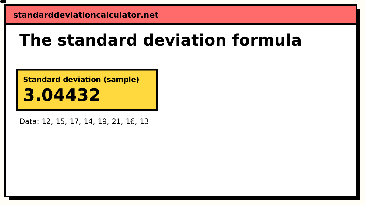
Standard deviation (sample)
3.04432
3.04
Your values typically sit about 3.04 above or below their mean of 15.88, in the same units as your data. 5 of 8 values (63%) fall between 12.83 and 18.92, within one standard deviation of the mean; for normally distributed data about 68% would.
Population SD (σ): 2.8477, if these values are the whole group.
- Count (n)
- 8
- Mean (x̄)
- 15.875
- Variance (s²)
- 9.26786
- Standard error
- 1.07633
- Minimum
- 12
- Q1 (25%)
- 13.75
- Median
- 15.5
- Q3 (75%)
- 17.5
- Maximum
- 21
- Range
- 9
More statistics (5)
- Relative SD (%RSD)
- 19.1768%
- Coefficient of variation
- 0.191768
- Sum (Σx)
- 127
- Sum of squares, Σ(x − x̄)²
- 64.875
- IQR (Q3 − Q1)
- 3.75
Data distribution
Shaded bands mark ±1, ±2 and ±3 SD from the mean. 5 of 8 values (63%) fall within ±1 SD.
Chart as text
Mean 15.875, sample standard deviation s = 3.04432, from 8 values between 12 and 21.
- Within ±1 SD (12.83 to 18.92): 5 of 8 values (63%). About 68% for normal data.
- Within ±2 SD: 8 (100%). About 95% for normal data.
- Within ±3 SD: 8 (100%). About 99.7% for normal data.
Show the working, step by step
Every term, explained
| Term | Name | What it does |
|---|---|---|
| x | Each value | Stands in turn for every individual number in your data. |
| x̄ / μ | Mean | The average: sample mean is written x̄ ("x-bar"), population mean μ ("mu"). |
| x − x̄ | Deviation | How far one value sits from the mean. Negative below it, positive above. |
| (x − x̄)² | Squared deviation | Makes every term positive so they cannot cancel, and penalises far-out values more. |
| Σ | Sum | "Add all of these up." |
| n / N | Count | How many values. Lower case n for a sample, capital N for a population. |
| n − 1 | Degrees of freedom | Bessel's correction (see below). |
| √ | Square root | Returns the answer to the original units after the squaring. |
Why square the deviations at all?
Try averaging the raw deviations on 2, 4, 6. The mean is 4, so the deviations are
−2, 0 and +2, and they sum to zero. That is not a coincidence of this example: the deviations
from the mean sum to zero for every dataset, by the definition of the mean. An
unsquared average of them would report zero spread for all data, which is useless.
Squaring solves that by making every term non-negative. It also has the side effect of weighting a deviation of 10 as a hundred times more significant than a deviation of 1, rather than ten times, which is why a single outlier can move a standard deviation so sharply. Taking the square root at the end undoes the inflation of scale, but not that reweighting.
Why n − 1 for a sample?
A sample's mean is calculated from that sample, so it sits as close to those particular numbers as any single point can. The true population mean is almost always somewhere slightly else, and further from your data on average. Measuring spread around the sample's own too-flattering centre therefore understates the population's real spread every time: the bias is systematic, not random.
Dividing by n − 1 instead of n inflates the result by exactly enough to cancel that bias out. The correction is named for Friedrich Bessel, and its size depends entirely on n:
| n | n / (n − 1) | Effect on the variance |
|---|---|---|
| 3 | 1.500 | 50% larger |
| 5 | 1.250 | 25% larger |
| 10 | 1.111 | 11% larger |
| 30 | 1.034 | 3.4% larger |
| 100 | 1.010 | 1% larger |
| 1000 | 1.001 | 0.1% larger |
For a large sample the choice barely matters. For a small one it matters a great deal, which is exactly when people are most likely to be working by hand and most likely to pick wrong.
A worked example, both ways
Data: 2, 4, 4, 4, 5, 5, 7, 9.
- Sum = 40, count = 8, so the mean is 5.
- Deviations: −3, −1, −1, −1, 0, 0, 2, 4.
- Squared: 9, 1, 1, 1, 0, 0, 4, 16. Their sum, Σ(x − x̄)², is 32.
-
As a population: 32 ÷ 8 = 4, and √4 = σ = 2 exactly.
As a sample: 32 ÷ 7 = 4.5714, and √4.5714 = s = 2.1381.
This is the standard textbook example precisely because the population answer comes out as a whole number. Paste it into the calculator above and toggle the mode to watch only the denominator change.
The empirical rule: 68%, 95%, 99.7%
When data follows a normal distribution, the familiar bell curve, the standard deviation predicts how much of the data sits near the centre:
- ±1σ captures about 68% of all values.
- ±2σ captures about 95% of all values.
- ±3σ captures about 99.7% of all values.
This is the empirical rule (or the 68-95-99.7 rule). It holds exactly for a normal distribution whatever its mean and σ, and only approximately for data that is roughly bell-shaped; skewed data can break it badly. A standard deviation graph shows how well it fits your own data, with the ±1σ, ±2σ and ±3σ bands drawn over the histogram.
It is also why outliers are often measured in standard deviations rather than raw units: under a normal distribution, a point beyond ±3σ sits in the outer 0.3%, which is why 3σ is a common cutoff.
The shortcut formula, and why not to use it
Older textbooks give a one-pass rearrangement that avoids computing the mean first:
s² = [ Σx² − (Σx)² / n ] / (n − 1)
Algebraically it is identical. Numerically it is not. It subtracts two large, nearly equal
quantities, and in floating-point arithmetic that step throws away most of the significant
digits. On the values 1000000.1, 1000000.2, 1000000.3 (whose true variance is
exactly 0.01), the shortcut can return zero or even a negative number, which is impossible
for a variance. The formulas at the top of this page, computed with
Welford's algorithm, do not have this failure mode.
Every standard deviation formula, in one table
The same idea rearranged for whatever you happen to have: raw values, a frequency table, several groups, or a variance somebody already computed.
| You want | Formula | Calculator |
|---|---|---|
| Sample SD | s = √[ Σ(x − x̄)² / (n − 1) ] | Standard deviation |
| Population SD | σ = √[ Σ(x − μ)² / N ] | Standard deviation |
| Variance | s² = Σ(x − x̄)² / (n − 1) | Variance |
| SD from a variance | s = √(s²) | Variance |
| Sum of squares | SS = Σ(x − x̄)² | Sum of squares |
| Standard error of the mean | SE = s / √n | Standard error |
| Relative SD (%RSD) | %RSD = 100 × s / |x̄| | Relative SD |
| Z-score | z = (x − μ) / σ | Z-score |
| Pooled SD | sp = √[ Σ(nᵢ − 1)sᵢ² / Σ(nᵢ − 1) ] | Pooled SD |
| Weighted SD | sw = √[ Σwᵢ(xᵢ − x̄w)² / (Σwᵢ − 1) ] | Weighted SD |
| Grouped frequency data | s = √[ Σf(x − x̄)² / (Σf − 1) ] | Grouped data |
| Mean absolute deviation | MAD = Σ|x − x̄| / n | MAD |
| Root mean square | RMS = √( Σx² / n ) | RMS |
| Binomial SD | σ = √( np(1 − p) ) | Binomial |
| Poisson SD | σ = √λ | Poisson |
| Two-asset portfolio SD | σp = √( w₁²σ₁² + w₂²σ₂² + 2w₁w₂ρσ₁σ₂ ) | Portfolio SD |
The formula for grouped data
When the data arrives as a frequency table rather than a list, you never see the individual values, only that some midpoint x occurred f times. Each squared deviation is therefore weighted by its frequency, and the count becomes Σf:
s = √[ Σf(x − x̄)² / (Σf − 1) ] where x̄ = Σfx / Σf
The answer is an approximation, because treating every value in a class as sitting exactly at the midpoint is a fiction: real values are spread across the interval. Expect it to run slightly low for heavily skewed classes. The grouped-data calculator shows the fx and fx² columns as it goes.
The formula to copy and paste (Word, Google Docs)
Plain Unicode, one line each, safe in Word, Google Docs, email or a comment:
s = √(Σ(x − x̄)² / (n − 1))σ = √(Σ(x − μ)² / N)
In LaTeX:
s = \sqrt{\frac{\sum (x_i - \bar{x})^2}{n-1}}\sigma = \sqrt{\frac{\sum (x_i - \mu)^2}{N}}
For a properly typeset version, both editors have an equation tool that accepts this syntax.
In Google Docs choose Insert → Equation and type
\sigma, \sqrt or \sum followed
by a space; each turns into its symbol. In Word, press
Alt+= to open an equation and paste the LaTeX line above; current
versions of Word convert it when you choose LaTeX in the Equation ribbon.
The notation guide has the individual characters and how to type each one.
The same formula in Excel, Python and R
Every one of these applies the formulas at the top of this page; they differ only in which denominator they pick by default, and that default is the single most common source of a wrong answer.
| Tool | Sample (n − 1) | Population (N) | Default |
|---|---|---|---|
| Excel, Sheets | =STDEV.S(A1:A100) | =STDEV.P(A1:A100) | Neither: you choose |
| NumPy | np.std(a, ddof=1) | np.std(a) | Population |
| pandas | s.std() | s.std(ddof=0) | Sample |
| Python statistics | statistics.stdev(a) | statistics.pstdev(a) | Neither: separate functions |
| R | sd(x) | sd(x) * sqrt((n − 1) / n) | Sample |
NumPy and pandas disagreeing on the default is a genuine trap: the same column run through
both returns two different numbers unless you set ddof explicitly. R has no
population function at all, so you rescale sd() by hand. The
Excel,
Python and
R guides work through each in full.
Related calculators
-
Standard deviation calculator
Apply the formula to your own numbers and see each step.
-
Symbols and notation
What σ, s, μ, x̄, n and Σ each stand for.
-
Sample vs population
Which denominator to use, and why it matters most for small n.
-
Variance calculator
The same formula without the final square root.
-
Variance formula
Sample, population, random-variable and grouped versions, each worked.
Common questions
What is the standard deviation formula?
For a sample: s = √[ Σ(x − x̄)² / (n − 1) ]. For a population:
σ = √[ Σ(x − μ)² / N ]. The two are identical except for the denominator:
a sample divides by n − 1, a population by N.
Why are the deviations squared?
Because deviations above and below the mean always sum to exactly zero, so averaging them raw would give 0 for every dataset. Squaring makes every term positive so they cannot cancel. It also weights large deviations more heavily than small ones, which is usually what you want from a measure of spread.
Taking absolute values instead would also stop the cancelling; that gives the mean absolute deviation, a real and occasionally preferable statistic. Squaring won out because it is differentiable everywhere and because variances of independent quantities add, which makes the whole of statistical theory tractable.
What is the computational or "shortcut" formula?
s² = [ Σx² − (Σx)²/n ] / (n − 1). It gives the same answer in exact
arithmetic and needs only one pass through the data, which mattered when people worked with
mechanical calculators.
On a computer it is a bad idea. It subtracts two large and nearly equal numbers, which destroys precision: on the data 1000000.1, 1000000.2, 1000000.3 it can return a negative variance. This site uses Welford's algorithm instead.
What does the Σ symbol mean in the formula?
Σ is the Greek capital sigma and means "add up all of these". Σ(x − x̄)²
instructs you to work out (x − x̄)² for every value x in the dataset and total the results.
The full notation guide is here.
Is the standard deviation formula the same as the variance formula?
Almost. The variance is everything under the square root; the standard deviation is the square root of it. So σ = √(σ²), and σ² = σ². The only practical difference is units: variance is in squared units, standard deviation is in the original units.
What is x in the standard deviation formula?
x represents each individual data point in the formula. In
s = √[ Σ(x − x̄)² / (n − 1) ], the instruction is: take every
value x in your dataset, subtract the sample mean (x̄) from it, square the result,
add all those squares together, then divide by n − 1 and take the square root. Some
textbooks write xᵢ (x-sub-i) to mean "the i-th data point" when working with sums.
Frequently asked questions about the standard deviation formula
Common questions
What do the symbols in the population standard deviation formula mean?
The population standard deviation formula is σ = √[ Σ(x − μ)² / N ]. The symbols are: σ = population SD, μ = population mean, x = each value, N = population size. The divisor is N because every member is included. See standard deviation formula for more detail.
Can you show the population standard deviation formula in plain text?
The population standard deviation formula is σ = √[ Σ(x − μ)² / N ]. The symbols are: σ = population SD, μ = population mean, x = each value, N = population size. The divisor is N because every member is included. See standard deviation formula for more detail.
What is the population standard deviation formula in Excel?
The population standard deviation formula is σ = √[ Σ(x − μ)² / N ]. The symbols are: σ = population SD, μ = population mean, x = each value, N = population size. The divisor is N because every member is included. See standard deviation formula for more detail.
What assumptions are used in the population standard deviation formula?
The population standard deviation formula is σ = √[ Σ(x − μ)² / N ]. The symbols are: σ = population SD, μ = population mean, x = each value, N = population size. The divisor is N because every member is included. See standard deviation formula for more detail.
How can I memorize the population standard deviation formula?
The population standard deviation formula is σ = √[ Σ(x − μ)² / N ]. The symbols are: σ = population SD, μ = population mean, x = each value, N = population size. The divisor is N because every member is included. See standard deviation formula for more detail.
Why does the sample population standard deviation formula use n minus 1?
The population standard deviation formula is σ = √[ Σ(x − μ)² / N ]. The symbols are: σ = population SD, μ = population mean, x = each value, N = population size. The divisor is N because every member is included. See standard deviation formula for more detail.
How do I rearrange the population standard deviation formula to solve for another variable?
The population standard deviation formula is σ = √[ Σ(x − μ)² / N ]. The symbols are: σ = population SD, μ = population mean, x = each value, N = population size. The divisor is N because every member is included. See standard deviation formula for more detail.
Can I see a worked example using the population standard deviation formula?
The population standard deviation formula is σ = √[ Σ(x − μ)² / N ]. The symbols are: σ = population SD, μ = population mean, x = each value, N = population size. The divisor is N because every member is included. See standard deviation formula for more detail.
What do the symbols in the sample standard deviation formula mean?
The sample standard deviation formula is s = √[ Σ(x − x̄)² / (n − 1) ]. Dividing by n − 1 (Bessel's correction) compensates for the fact that the sample mean is always closer to the sample values than the true population mean. See standard deviation formula for a term-by-term breakdown.
Can you show the sample standard deviation formula in plain text?
The sample standard deviation formula is s = √[ Σ(x − x̄)² / (n − 1) ]. Dividing by n − 1 (Bessel's correction) compensates for the fact that the sample mean is always closer to the sample values than the true population mean. See standard deviation formula for a term-by-term breakdown.
What is the sample standard deviation formula in Excel?
The sample standard deviation formula is s = √[ Σ(x − x̄)² / (n − 1) ]. Dividing by n − 1 (Bessel's correction) compensates for the fact that the sample mean is always closer to the sample values than the true population mean. See standard deviation formula for a term-by-term breakdown.
What assumptions are used in the sample standard deviation formula?
The sample standard deviation formula is s = √[ Σ(x − x̄)² / (n − 1) ]. Dividing by n − 1 (Bessel's correction) compensates for the fact that the sample mean is always closer to the sample values than the true population mean. See standard deviation formula for a term-by-term breakdown.
How can I memorize the sample standard deviation formula?
The sample standard deviation formula is s = √[ Σ(x − x̄)² / (n − 1) ]. Dividing by n − 1 (Bessel's correction) compensates for the fact that the sample mean is always closer to the sample values than the true population mean. See standard deviation formula for a term-by-term breakdown.
Why does the sample sample standard deviation formula use n minus 1?
The sample standard deviation formula is s = √[ Σ(x − x̄)² / (n − 1) ]. Dividing by n − 1 (Bessel's correction) compensates for the fact that the sample mean is always closer to the sample values than the true population mean. See standard deviation formula for a term-by-term breakdown.
How do I rearrange the sample standard deviation formula to solve for another variable?
The sample standard deviation formula is s = √[ Σ(x − x̄)² / (n − 1) ]. Dividing by n − 1 (Bessel's correction) compensates for the fact that the sample mean is always closer to the sample values than the true population mean. See standard deviation formula for a term-by-term breakdown.
Can I see a worked example using the sample standard deviation formula?
The sample standard deviation formula is s = √[ Σ(x − x̄)² / (n − 1) ]. Dividing by n − 1 (Bessel's correction) compensates for the fact that the sample mean is always closer to the sample values than the true population mean. See standard deviation formula for a term-by-term breakdown.
Can you show the standard deviation formula in plain text?
The sample standard deviation formula is s = √[Σ(x − x̄)² / (n − 1)]. The population formula is identical except the denominator is N instead of n − 1. The Σ symbol means 'sum up'. See standard deviation formula for a term-by-term breakdown.
What is the standard deviation formula in Excel?
The sample standard deviation formula is s = √[Σ(x − x̄)² / (n − 1)]. The population formula is identical except the denominator is N instead of n − 1. The Σ symbol means 'sum up'. See standard deviation formula for a term-by-term breakdown.
How can I memorize the standard deviation formula?
The sample standard deviation formula is s = √[Σ(x − x̄)² / (n − 1)]. The population formula is identical except the denominator is N instead of n − 1. The Σ symbol means 'sum up'. See standard deviation formula for a term-by-term breakdown.
Why does the sample standard deviation formula use n minus 1?
The sample standard deviation formula is s = √[ Σ(x − x̄)² / (n − 1) ]. Dividing by n − 1 (Bessel's correction) compensates for the fact that the sample mean is always closer to the sample values than the true population mean. See standard deviation formula for a term-by-term breakdown.
How do I rearrange the standard deviation formula to solve for another variable?
The sample standard deviation formula is s = √[Σ(x − x̄)² / (n − 1)]. The population formula is identical except the denominator is N instead of n − 1. The Σ symbol means 'sum up'. See standard deviation formula for a term-by-term breakdown.
Can I see a worked example using the standard deviation formula?
The sample standard deviation formula is s = √[Σ(x − x̄)² / (n − 1)]. The population formula is identical except the denominator is N instead of n − 1. The Σ symbol means 'sum up'. See standard deviation formula for a term-by-term breakdown.
What should a beginner know about the sample standard deviation formula?
The sample standard deviation formula is s = √[ Σ(x − x̄)² / (n − 1) ]. Dividing by n − 1 (Bessel's correction) compensates for the fact that the sample mean is always closer to the sample values than the true population mean. See standard deviation formula for a term-by-term breakdown.
What should a beginner know about the population standard deviation formula?
The population standard deviation formula is σ = √[ Σ(x − μ)² / N ]. The symbols are: σ = population SD, μ = population mean, x = each value, N = population size. The divisor is N because every member is included. See standard deviation formula for more detail.
What should a high-school student know about the sample standard deviation formula?
The sample standard deviation formula is s = √[ Σ(x − x̄)² / (n − 1) ]. Dividing by n − 1 (Bessel's correction) compensates for the fact that the sample mean is always closer to the sample values than the true population mean. See standard deviation formula for a term-by-term breakdown.
What should a high-school student know about the population standard deviation formula?
The population standard deviation formula is σ = √[ Σ(x − μ)² / N ]. The symbols are: σ = population SD, μ = population mean, x = each value, N = population size. The divisor is N because every member is included. See standard deviation formula for more detail.
What should a college student know about the sample standard deviation formula?
The sample standard deviation formula is s = √[ Σ(x − x̄)² / (n − 1) ]. Dividing by n − 1 (Bessel's correction) compensates for the fact that the sample mean is always closer to the sample values than the true population mean. See standard deviation formula for a term-by-term breakdown.
What should a college student know about the population standard deviation formula?
The population standard deviation formula is σ = √[ Σ(x − μ)² / N ]. The symbols are: σ = population SD, μ = population mean, x = each value, N = population size. The divisor is N because every member is included. See standard deviation formula for more detail.
What should a researcher know about the sample standard deviation formula?
The sample standard deviation formula is s = √[ Σ(x − x̄)² / (n − 1) ]. Dividing by n − 1 (Bessel's correction) compensates for the fact that the sample mean is always closer to the sample values than the true population mean. See standard deviation formula for a term-by-term breakdown.
What should a researcher know about the population standard deviation formula?
The population standard deviation formula is σ = √[ Σ(x − μ)² / N ]. The symbols are: σ = population SD, μ = population mean, x = each value, N = population size. The divisor is N because every member is included. See standard deviation formula for more detail.
What should a data analyst know about the sample standard deviation formula?
The sample standard deviation formula is s = √[ Σ(x − x̄)² / (n − 1) ]. Dividing by n − 1 (Bessel's correction) compensates for the fact that the sample mean is always closer to the sample values than the true population mean. See standard deviation formula for a term-by-term breakdown.
What should a data analyst know about the population standard deviation formula?
The population standard deviation formula is σ = √[ Σ(x − μ)² / N ]. The symbols are: σ = population SD, μ = population mean, x = each value, N = population size. The divisor is N because every member is included. See standard deviation formula for more detail.
What should a teacher preparing a lesson know about the sample standard deviation formula?
The sample standard deviation formula is s = √[ Σ(x − x̄)² / (n − 1) ]. Dividing by n − 1 (Bessel's correction) compensates for the fact that the sample mean is always closer to the sample values than the true population mean. See standard deviation formula for a term-by-term breakdown.
What should a teacher preparing a lesson know about the population standard deviation formula?
The population standard deviation formula is σ = √[ Σ(x − μ)² / N ]. The symbols are: σ = population SD, μ = population mean, x = each value, N = population size. The divisor is N because every member is included. See standard deviation formula for more detail.
What should someone preparing for a statistics exam know about the sample standard deviation formula?
The sample standard deviation formula is s = √[ Σ(x − x̄)² / (n − 1) ]. Dividing by n − 1 (Bessel's correction) compensates for the fact that the sample mean is always closer to the sample values than the true population mean. See standard deviation formula for a term-by-term breakdown.
What should someone preparing for a statistics exam know about the population standard deviation formula?
The population standard deviation formula is σ = √[ Σ(x − μ)² / N ]. The symbols are: σ = population SD, μ = population mean, x = each value, N = population size. The divisor is N because every member is included. See standard deviation formula for more detail.
What should a business analyst know about the sample standard deviation formula?
The sample standard deviation formula is s = √[ Σ(x − x̄)² / (n − 1) ]. Dividing by n − 1 (Bessel's correction) compensates for the fact that the sample mean is always closer to the sample values than the true population mean. See standard deviation formula for a term-by-term breakdown.
What should a business analyst know about the population standard deviation formula?
The population standard deviation formula is σ = √[ Σ(x − μ)² / N ]. The symbols are: σ = population SD, μ = population mean, x = each value, N = population size. The divisor is N because every member is included. See standard deviation formula for more detail.
What should a quality-control engineer know about the sample standard deviation formula?
The sample standard deviation formula is s = √[ Σ(x − x̄)² / (n − 1) ]. Dividing by n − 1 (Bessel's correction) compensates for the fact that the sample mean is always closer to the sample values than the true population mean. See standard deviation formula for a term-by-term breakdown.
What is the formula for sample standard deviation?
The sample standard deviation formula is s = √[ Σ(x − x̄)² / (n − 1) ]. Dividing by n − 1 (Bessel's correction) compensates for the fact that the sample mean is always closer to the sample values than the true population mean. See standard deviation formula for a term-by-term breakdown.
How do you derive the formula for sample standard deviation?
The sample standard deviation formula is s = √[ Σ(x − x̄)² / (n − 1) ]. Dividing by n − 1 (Bessel's correction) compensates for the fact that the sample mean is always closer to the sample values than the true population mean. See standard deviation formula for a term-by-term breakdown.
When should I use the formula for sample standard deviation?
The sample standard deviation formula is s = √[ Σ(x − x̄)² / (n − 1) ]. Dividing by n − 1 (Bessel's correction) compensates for the fact that the sample mean is always closer to the sample values than the true population mean. See standard deviation formula for a term-by-term breakdown.
What is the Google Sheets formula for sample standard deviation?
The sample standard deviation formula is s = √[ Σ(x − x̄)² / (n − 1) ]. Dividing by n − 1 (Bessel's correction) compensates for the fact that the sample mean is always closer to the sample values than the true population mean. See standard deviation formula for a term-by-term breakdown.
What is the Python formula for sample standard deviation?
The sample standard deviation formula is s = √[ Σ(x − x̄)² / (n − 1) ]. Dividing by n − 1 (Bessel's correction) compensates for the fact that the sample mean is always closer to the sample values than the true population mean. See standard deviation formula for a term-by-term breakdown.
What is the R formula for sample standard deviation?
The sample standard deviation formula is s = √[ Σ(x − x̄)² / (n − 1) ]. Dividing by n − 1 (Bessel's correction) compensates for the fact that the sample mean is always closer to the sample values than the true population mean. See standard deviation formula for a term-by-term breakdown.
What is the JavaScript formula for sample standard deviation?
The sample standard deviation formula is s = √[ Σ(x − x̄)² / (n − 1) ]. Dividing by n − 1 (Bessel's correction) compensates for the fact that the sample mean is always closer to the sample values than the true population mean. See standard deviation formula for a term-by-term breakdown.
What is the Java formula for sample standard deviation?
The sample standard deviation formula is s = √[ Σ(x − x̄)² / (n − 1) ]. Dividing by n − 1 (Bessel's correction) compensates for the fact that the sample mean is always closer to the sample values than the true population mean. See standard deviation formula for a term-by-term breakdown.
What is the C++ formula for sample standard deviation?
The sample standard deviation formula is s = √[ Σ(x − x̄)² / (n − 1) ]. Dividing by n − 1 (Bessel's correction) compensates for the fact that the sample mean is always closer to the sample values than the true population mean. See standard deviation formula for a term-by-term breakdown.
What is the SQL formula for sample standard deviation?
The sample standard deviation formula is s = √[ Σ(x − x̄)² / (n − 1) ]. Dividing by n − 1 (Bessel's correction) compensates for the fact that the sample mean is always closer to the sample values than the true population mean. See standard deviation formula for a term-by-term breakdown.
What is the formula for standard error of the mean?
The standard error of the mean formula is SE = s / √n. Use the standard error calculator for computation.
How do you derive the formula for standard error of the mean?
The standard error of the mean formula is SE = s / √n. Use the standard error calculator for computation.
When should I use the formula for standard error of the mean?
The standard error of the mean formula is SE = s / √n. Use the standard error calculator for computation.
Can you show the standard error of the mean formula in plain text?
The standard error of the mean formula is SE = s / √n. Use the standard error calculator for computation.
What is the standard error of the mean formula in Excel?
The standard error of the mean formula is SE = s / √n. Use the standard error calculator for computation.
What is the standard error of the mean formula for grouped data?
The standard error of the mean formula is SE = s / √n. Use the standard error calculator for computation.
What assumptions are used in the standard error of the mean formula?
The standard error of the mean formula is SE = s / √n. Use the standard error calculator for computation.
How can I memorize the standard error of the mean formula?
The standard error of the mean formula is SE = s / √n. Use the standard error calculator for computation.
What is the difference between the sample and population standard error of the mean formulas?
The population standard deviation formula is σ = √[ Σ(x − μ)² / N ]. The symbols are: σ = population SD, μ = population mean, x = each value, N = population size. The divisor is N because every member is included. See standard deviation formula for more detail.
Why does the sample standard error of the mean formula use n minus 1?
The sample standard deviation formula is s = √[ Σ(x − x̄)² / (n − 1) ]. Dividing by n − 1 (Bessel's correction) compensates for the fact that the sample mean is always closer to the sample values than the true population mean. See standard deviation formula for a term-by-term breakdown.
How do I rearrange the standard error of the mean formula to solve for another variable?
The standard error of the mean formula is SE = s / √n. Use the standard error calculator for computation.
Can I see a worked example using the standard error of the mean formula?
The standard error of the mean formula is SE = s / √n. Use the standard error calculator for computation.
What do the symbols in the relative standard deviation formula mean?
The relative standard deviation formula is RSD = (s / x̄) × 100%. The coefficient of variation is the same without × 100: CV = s / x̄. Use the relative standard deviation calculator for computation.
Can you show the relative standard deviation formula in plain text?
The relative standard deviation formula is RSD = (s / x̄) × 100%. The coefficient of variation is the same without × 100: CV = s / x̄. Use the relative standard deviation calculator for computation.
What is the relative standard deviation formula in Excel?
The relative standard deviation formula is RSD = (s / x̄) × 100%. The coefficient of variation is the same without × 100: CV = s / x̄. Use the relative standard deviation calculator for computation.
What is the relative standard deviation formula for grouped data?
The relative standard deviation formula is RSD = (s / x̄) × 100%. The coefficient of variation is the same without × 100: CV = s / x̄. Use the relative standard deviation calculator for computation.
Does the relative standard deviation formula change for a sample?
The sample standard deviation formula is s = √[ Σ(x − x̄)² / (n − 1) ]. Dividing by n − 1 (Bessel's correction) compensates for the fact that the sample mean is always closer to the sample values than the true population mean. See standard deviation formula for a term-by-term breakdown.
What assumptions are used in the relative standard deviation formula?
The relative standard deviation formula is RSD = (s / x̄) × 100%. The coefficient of variation is the same without × 100: CV = s / x̄. Use the relative standard deviation calculator for computation.
How can I memorize the relative standard deviation formula?
The relative standard deviation formula is RSD = (s / x̄) × 100%. The coefficient of variation is the same without × 100: CV = s / x̄. Use the relative standard deviation calculator for computation.
Why does the sample relative standard deviation formula use n minus 1?
The sample standard deviation formula is s = √[ Σ(x − x̄)² / (n − 1) ]. Dividing by n − 1 (Bessel's correction) compensates for the fact that the sample mean is always closer to the sample values than the true population mean. See standard deviation formula for a term-by-term breakdown.
How do I rearrange the relative standard deviation formula to solve for another variable?
The relative standard deviation formula is RSD = (s / x̄) × 100%. The coefficient of variation is the same without × 100: CV = s / x̄. Use the relative standard deviation calculator for computation.
Can I see a worked example using the relative standard deviation formula?
The relative standard deviation formula is RSD = (s / x̄) × 100%. The coefficient of variation is the same without × 100: CV = s / x̄. Use the relative standard deviation calculator for computation.
What is the relative standard deviation formula?
The relative standard deviation formula is RSD = (s / x̄) × 100%. The coefficient of variation is the same without × 100: CV = s / x̄. Use the relative standard deviation calculator for computation.
Can you copy and paste the population standard deviation equation?
The population standard deviation formula is σ = √[ Σ(x − μ)² / N ]. The symbols are: σ = population SD, μ = population mean, x = each value, N = population size. The divisor is N because every member is included. See standard deviation formula for more detail.
Can you copy and paste the sample standard deviation equation?
The sample standard deviation formula is s = √[ Σ(x − x̄)² / (n − 1) ]. Dividing by n − 1 (Bessel's correction) compensates for the fact that the sample mean is always closer to the sample values than the true population mean. See standard deviation formula for a term-by-term breakdown.
Can you copy and paste the standard deviation equation?
The sample standard deviation formula is s = √[Σ(x − x̄)² / (n − 1)]. The population formula is identical except the denominator is N instead of n − 1. The Σ symbol means 'sum up'. See standard deviation formula for a term-by-term breakdown.
Can you copy and paste the variance equation?
The variance formula is s² = Σ(x − x̄)² / (n − 1) for a sample. The standard deviation is the square root of the variance. The computational formula s² = [Σx² − (Σx)²/n] / (n − 1) is mathematically equivalent but should not be used on a computer due to precision loss. See standard deviation formula for a full derivation.
Can you copy and paste the coefficient of variation equation?
The relative standard deviation formula is RSD = (s / x̄) × 100%. The coefficient of variation is the same without × 100: CV = s / x̄. Use the relative standard deviation calculator for computation.
Can you copy and paste the pooled standard deviation equation?
The pooled standard deviation formula combines two or more groups: s_p = √[ Σ(n_i − 1)s_i² / Σ(n_i − 1) ]. Use the pooled standard deviation calculator for computation.
How do I calculate standard deviation for a filtered dataset in Excel?
The sample standard deviation formula is s = √[Σ(x − x̄)² / (n − 1)]. The population formula is identical except the denominator is N instead of n − 1. The Σ symbol means 'sum up'. See standard deviation formula for a term-by-term breakdown.
How do I calculate standard deviation in Google Sheets?
The sample standard deviation formula is s = √[Σ(x − x̄)² / (n − 1)]. The population formula is identical except the denominator is N instead of n − 1. The Σ symbol means 'sum up'. See standard deviation formula for a term-by-term breakdown.
How do I calculate standard deviation for a filtered dataset in Google Sheets?
The sample standard deviation formula is s = √[Σ(x − x̄)² / (n − 1)]. The population formula is identical except the denominator is N instead of n − 1. The Σ symbol means 'sum up'. See standard deviation formula for a term-by-term breakdown.
Why does the sample variance formula use n minus 1?
The variance formula is s² = Σ(x − x̄)² / (n − 1) for a sample. The standard deviation is the square root of the variance. The computational formula s² = [Σx² − (Σx)²/n] / (n − 1) is mathematically equivalent but should not be used on a computer due to precision loss. See standard deviation formula for a full derivation.
What is the formula for standard deviation?
The sample standard deviation formula is s = √[Σ(x − x̄)² / (n − 1)]. The population formula is identical except the denominator is N instead of n − 1. The Σ symbol means 'sum up'. See standard deviation formula for a term-by-term breakdown.
How do you derive the formula for standard deviation?
The sample standard deviation formula is s = √[Σ(x − x̄)² / (n − 1)]. The population formula is identical except the denominator is N instead of n − 1. The Σ symbol means 'sum up'. See standard deviation formula for a term-by-term breakdown.
When should I use the formula for standard deviation?
The sample standard deviation formula is s = √[Σ(x − x̄)² / (n − 1)]. The population formula is identical except the denominator is N instead of n − 1. The Σ symbol means 'sum up'. See standard deviation formula for a term-by-term breakdown.
What is the formula for pooled standard deviation?
The pooled standard deviation formula combines two or more groups: s_p = √[ Σ(n_i − 1)s_i² / Σ(n_i − 1) ]. Use the pooled standard deviation calculator for computation.
How do you derive the formula for pooled standard deviation?
The pooled standard deviation formula combines two or more groups: s_p = √[ Σ(n_i − 1)s_i² / Σ(n_i − 1) ]. Use the pooled standard deviation calculator for computation.
When should I use the formula for pooled standard deviation?
The pooled standard deviation formula combines two or more groups: s_p = √[ Σ(n_i − 1)s_i² / Σ(n_i − 1) ]. Use the pooled standard deviation calculator for computation.
What do the symbols in the pooled standard deviation formula mean?
The pooled standard deviation formula combines two or more groups: s_p = √[ Σ(n_i − 1)s_i² / Σ(n_i − 1) ]. Use the pooled standard deviation calculator for computation.
Can you show the pooled standard deviation formula in plain text?
The pooled standard deviation formula combines two or more groups: s_p = √[ Σ(n_i − 1)s_i² / Σ(n_i − 1) ]. Use the pooled standard deviation calculator for computation.
What is the pooled standard deviation formula in Excel?
The pooled standard deviation formula combines two or more groups: s_p = √[ Σ(n_i − 1)s_i² / Σ(n_i − 1) ]. Use the pooled standard deviation calculator for computation.
What is the pooled standard deviation formula for grouped data?
The pooled standard deviation formula combines two or more groups: s_p = √[ Σ(n_i − 1)s_i² / Σ(n_i − 1) ]. Use the pooled standard deviation calculator for computation.
Does the pooled standard deviation formula change for a sample?
The sample standard deviation formula is s = √[ Σ(x − x̄)² / (n − 1) ]. Dividing by n − 1 (Bessel's correction) compensates for the fact that the sample mean is always closer to the sample values than the true population mean. See standard deviation formula for a term-by-term breakdown.
What assumptions are used in the pooled standard deviation formula?
The pooled standard deviation formula combines two or more groups: s_p = √[ Σ(n_i − 1)s_i² / Σ(n_i − 1) ]. Use the pooled standard deviation calculator for computation.
How can I memorize the pooled standard deviation formula?
The pooled standard deviation formula combines two or more groups: s_p = √[ Σ(n_i − 1)s_i² / Σ(n_i − 1) ]. Use the pooled standard deviation calculator for computation.
Why does the sample pooled standard deviation formula use n minus 1?
The sample standard deviation formula is s = √[ Σ(x − x̄)² / (n − 1) ]. Dividing by n − 1 (Bessel's correction) compensates for the fact that the sample mean is always closer to the sample values than the true population mean. See standard deviation formula for a term-by-term breakdown.
How do I rearrange the pooled standard deviation formula to solve for another variable?
The pooled standard deviation formula combines two or more groups: s_p = √[ Σ(n_i − 1)s_i² / Σ(n_i − 1) ]. Use the pooled standard deviation calculator for computation.
Can I see a worked example using the pooled standard deviation formula?
The pooled standard deviation formula combines two or more groups: s_p = √[ Σ(n_i − 1)s_i² / Σ(n_i − 1) ]. Use the pooled standard deviation calculator for computation.
How do I calculate standard deviation in Excel?
The sample standard deviation formula is s = √[Σ(x − x̄)² / (n − 1)]. The population formula is identical except the denominator is N instead of n − 1. The Σ symbol means 'sum up'. See standard deviation formula for a term-by-term breakdown.
How do I calculate variance and standard deviation in Excel?
The variance formula is s² = Σ(x − x̄)² / (n − 1) for a sample. The standard deviation is the square root of the variance. The computational formula s² = [Σx² − (Σx)²/n] / (n − 1) is mathematically equivalent but should not be used on a computer due to precision loss. See standard deviation formula for a full derivation.
How do I handle blank cells when calculating standard deviation in Excel?
The sample standard deviation formula is s = √[Σ(x − x̄)² / (n − 1)]. The population formula is identical except the denominator is N instead of n − 1. The Σ symbol means 'sum up'. See standard deviation formula for a term-by-term breakdown.
What do the symbols in the variance formula mean?
The variance formula is s² = Σ(x − x̄)² / (n − 1) for a sample. The standard deviation is the square root of the variance. The computational formula s² = [Σx² − (Σx)²/n] / (n − 1) is mathematically equivalent but should not be used on a computer due to precision loss. See standard deviation formula for a full derivation.
What do the symbols in the standard deviation formula mean?
The sample standard deviation formula is s = √[Σ(x − x̄)² / (n − 1)]. The population formula is identical except the denominator is N instead of n − 1. The Σ symbol means 'sum up'. See standard deviation formula for a term-by-term breakdown.
What do the symbols in the standard error of the mean formula mean?
The standard error of the mean formula is SE = s / √n. Use the standard error calculator for computation.
How can I check a Excel standard deviation result with an online calculator?
The sample standard deviation formula is s = √[Σ(x − x̄)² / (n − 1)]. The population formula is identical except the denominator is N instead of n − 1. The Σ symbol means 'sum up'. See standard deviation formula for a term-by-term breakdown.
Which formula should I use for standard deviation with a dataset with percentages?
The sample standard deviation formula is s = √[Σ(x − x̄)² / (n − 1)]. The population formula is identical except the denominator is N instead of n − 1. The Σ symbol means 'sum up'. See standard deviation formula for a term-by-term breakdown.
What is the formula for relative standard deviation?
The relative standard deviation formula is RSD = (s / x̄) × 100%. The coefficient of variation is the same without × 100: CV = s / x̄. Use the relative standard deviation calculator for computation.
How do you derive the formula for relative standard deviation?
The relative standard deviation formula is RSD = (s / x̄) × 100%. The coefficient of variation is the same without × 100: CV = s / x̄. Use the relative standard deviation calculator for computation.
When should I use the formula for relative standard deviation?
The relative standard deviation formula is RSD = (s / x̄) × 100%. The coefficient of variation is the same without × 100: CV = s / x̄. Use the relative standard deviation calculator for computation.
Can you copy and paste the standard error of the mean equation?
The standard error of the mean formula is SE = s / √n. Use the standard error calculator for computation.
What is the formula for coefficient of variation?
The relative standard deviation formula is RSD = (s / x̄) × 100%. The coefficient of variation is the same without × 100: CV = s / x̄. Use the relative standard deviation calculator for computation.
How do you derive the formula for coefficient of variation?
The relative standard deviation formula is RSD = (s / x̄) × 100%. The coefficient of variation is the same without × 100: CV = s / x̄. Use the relative standard deviation calculator for computation.
When should I use the formula for coefficient of variation?
The relative standard deviation formula is RSD = (s / x̄) × 100%. The coefficient of variation is the same without × 100: CV = s / x̄. Use the relative standard deviation calculator for computation.
What do the symbols in the coefficient of variation formula mean?
The relative standard deviation formula is RSD = (s / x̄) × 100%. The coefficient of variation is the same without × 100: CV = s / x̄. Use the relative standard deviation calculator for computation.
Can you show the coefficient of variation formula in plain text?
The relative standard deviation formula is RSD = (s / x̄) × 100%. The coefficient of variation is the same without × 100: CV = s / x̄. Use the relative standard deviation calculator for computation.
What is the coefficient of variation formula in Excel?
The relative standard deviation formula is RSD = (s / x̄) × 100%. The coefficient of variation is the same without × 100: CV = s / x̄. Use the relative standard deviation calculator for computation.
What is the coefficient of variation formula for grouped data?
The relative standard deviation formula is RSD = (s / x̄) × 100%. The coefficient of variation is the same without × 100: CV = s / x̄. Use the relative standard deviation calculator for computation.
Does the coefficient of variation formula change for a sample?
The sample standard deviation formula is s = √[ Σ(x − x̄)² / (n − 1) ]. Dividing by n − 1 (Bessel's correction) compensates for the fact that the sample mean is always closer to the sample values than the true population mean. See standard deviation formula for a term-by-term breakdown.
What assumptions are used in the coefficient of variation formula?
The relative standard deviation formula is RSD = (s / x̄) × 100%. The coefficient of variation is the same without × 100: CV = s / x̄. Use the relative standard deviation calculator for computation.
How can I memorize the coefficient of variation formula?
The relative standard deviation formula is RSD = (s / x̄) × 100%. The coefficient of variation is the same without × 100: CV = s / x̄. Use the relative standard deviation calculator for computation.
What is the difference between the sample and population coefficient of variation formulas?
The population standard deviation formula is σ = √[ Σ(x − μ)² / N ]. The symbols are: σ = population SD, μ = population mean, x = each value, N = population size. The divisor is N because every member is included. See standard deviation formula for more detail.
Why does the sample coefficient of variation formula use n minus 1?
The sample standard deviation formula is s = √[ Σ(x − x̄)² / (n − 1) ]. Dividing by n − 1 (Bessel's correction) compensates for the fact that the sample mean is always closer to the sample values than the true population mean. See standard deviation formula for a term-by-term breakdown.
How do I rearrange the coefficient of variation formula to solve for another variable?
The relative standard deviation formula is RSD = (s / x̄) × 100%. The coefficient of variation is the same without × 100: CV = s / x̄. Use the relative standard deviation calculator for computation.
Can I see a worked example using the coefficient of variation formula?
The relative standard deviation formula is RSD = (s / x̄) × 100%. The coefficient of variation is the same without × 100: CV = s / x̄. Use the relative standard deviation calculator for computation.
Can you copy and paste the relative standard deviation equation?
The relative standard deviation formula is RSD = (s / x̄) × 100%. The coefficient of variation is the same without × 100: CV = s / x̄. Use the relative standard deviation calculator for computation.
Which formula should I use for standard deviation with weighted observations?
The sample standard deviation formula is s = √[Σ(x − x̄)² / (n − 1)]. The population formula is identical except the denominator is N instead of n − 1. The Σ symbol means 'sum up'. See standard deviation formula for a term-by-term breakdown.
What is the difference between the sample and population population standard deviation formulas?
The population standard deviation formula is σ = √[ Σ(x − μ)² / N ]. The symbols are: σ = population SD, μ = population mean, x = each value, N = population size. The divisor is N because every member is included. See standard deviation formula for more detail.
What is the difference between the sample and population sample standard deviation formulas?
The population standard deviation formula is σ = √[ Σ(x − μ)² / N ]. The symbols are: σ = population SD, μ = population mean, x = each value, N = population size. The divisor is N because every member is included. See standard deviation formula for more detail.
What is the difference between the sample and population standard deviation formulas?
The population standard deviation formula is σ = √[ Σ(x − μ)² / N ]. The symbols are: σ = population SD, μ = population mean, x = each value, N = population size. The divisor is N because every member is included. See standard deviation formula for more detail.
What is the difference between the sample and population relative standard deviation formulas?
The population standard deviation formula is σ = √[ Σ(x − μ)² / N ]. The symbols are: σ = population SD, μ = population mean, x = each value, N = population size. The divisor is N because every member is included. See standard deviation formula for more detail.
What is the difference between the sample and population pooled standard deviation formulas?
The population standard deviation formula is σ = √[ Σ(x − μ)² / N ]. The symbols are: σ = population SD, μ = population mean, x = each value, N = population size. The divisor is N because every member is included. See standard deviation formula for more detail.
What is the formula for population standard deviation?
The population standard deviation formula is σ = √[ Σ(x − μ)² / N ]. The symbols are: σ = population SD, μ = population mean, x = each value, N = population size. The divisor is N because every member is included. See standard deviation formula for more detail.
How do you derive the formula for population standard deviation?
The population standard deviation formula is σ = √[ Σ(x − μ)² / N ]. The symbols are: σ = population SD, μ = population mean, x = each value, N = population size. The divisor is N because every member is included. See standard deviation formula for more detail.
When should I use the formula for population standard deviation?
The population standard deviation formula is σ = √[ Σ(x − μ)² / N ]. The symbols are: σ = population SD, μ = population mean, x = each value, N = population size. The divisor is N because every member is included. See standard deviation formula for more detail.
What is the Google Sheets formula for population standard deviation?
The population standard deviation formula is σ = √[ Σ(x − μ)² / N ]. The symbols are: σ = population SD, μ = population mean, x = each value, N = population size. The divisor is N because every member is included. See standard deviation formula for more detail.
What is the Python formula for population standard deviation?
The population standard deviation formula is σ = √[ Σ(x − μ)² / N ]. The symbols are: σ = population SD, μ = population mean, x = each value, N = population size. The divisor is N because every member is included. See standard deviation formula for more detail.
What is the R formula for population standard deviation?
The population standard deviation formula is σ = √[ Σ(x − μ)² / N ]. The symbols are: σ = population SD, μ = population mean, x = each value, N = population size. The divisor is N because every member is included. See standard deviation formula for more detail.
What is the JavaScript formula for population standard deviation?
The population standard deviation formula is σ = √[ Σ(x − μ)² / N ]. The symbols are: σ = population SD, μ = population mean, x = each value, N = population size. The divisor is N because every member is included. See standard deviation formula for more detail.
What is the Java formula for population standard deviation?
The population standard deviation formula is σ = √[ Σ(x − μ)² / N ]. The symbols are: σ = population SD, μ = population mean, x = each value, N = population size. The divisor is N because every member is included. See standard deviation formula for more detail.
What is the C++ formula for population standard deviation?
The population standard deviation formula is σ = √[ Σ(x − μ)² / N ]. The symbols are: σ = population SD, μ = population mean, x = each value, N = population size. The divisor is N because every member is included. See standard deviation formula for more detail.
What is the SQL formula for population standard deviation?
The population standard deviation formula is σ = √[ Σ(x − μ)² / N ]. The symbols are: σ = population SD, μ = population mean, x = each value, N = population size. The divisor is N because every member is included. See standard deviation formula for more detail.
What is the difference between the sample and population variance formulas?
The variance formula is s² = Σ(x − x̄)² / (n − 1) for a sample. The standard deviation is the square root of the variance. The computational formula s² = [Σx² − (Σx)²/n] / (n − 1) is mathematically equivalent but should not be used on a computer due to precision loss. See standard deviation formula for a full derivation.
What assumptions are used in the standard deviation formula?
The sample standard deviation formula is s = √[Σ(x − x̄)² / (n − 1)]. The population formula is identical except the denominator is N instead of n − 1. The Σ symbol means 'sum up'. See standard deviation formula for a term-by-term breakdown.
What is the formula for variance?
The variance formula is s² = Σ(x − x̄)² / (n − 1) for a sample. The standard deviation is the square root of the variance. The computational formula s² = [Σx² − (Σx)²/n] / (n − 1) is mathematically equivalent but should not be used on a computer due to precision loss. See standard deviation formula for a full derivation.
How do you derive the formula for variance?
The variance formula is s² = Σ(x − x̄)² / (n − 1) for a sample. The standard deviation is the square root of the variance. The computational formula s² = [Σx² − (Σx)²/n] / (n − 1) is mathematically equivalent but should not be used on a computer due to precision loss. See standard deviation formula for a full derivation.
How do I calculate variance and standard deviation in Google Sheets?
The variance formula is s² = Σ(x − x̄)² / (n − 1) for a sample. The standard deviation is the square root of the variance. The computational formula s² = [Σx² − (Σx)²/n] / (n − 1) is mathematically equivalent but should not be used on a computer due to precision loss. See standard deviation formula for a full derivation.
What is the Excel formula for sample standard deviation?
The sample standard deviation formula is s = √[ Σ(x − x̄)² / (n − 1) ]. Dividing by n − 1 (Bessel's correction) compensates for the fact that the sample mean is always closer to the sample values than the true population mean. See standard deviation formula for a term-by-term breakdown.
What is the Excel formula for population standard deviation?
The population standard deviation formula is σ = √[ Σ(x − μ)² / N ]. The symbols are: σ = population SD, μ = population mean, x = each value, N = population size. The divisor is N because every member is included. See standard deviation formula for more detail.
How do I calculate standard deviation from a frequency table in Excel?
The sample standard deviation formula is s = √[Σ(x − x̄)² / (n − 1)]. The population formula is identical except the denominator is N instead of n − 1. The Σ symbol means 'sum up'. See standard deviation formula for a term-by-term breakdown.
How do I handle blank cells when calculating standard deviation in Google Sheets?
The sample standard deviation formula is s = √[Σ(x − x̄)² / (n − 1)]. The population formula is identical except the denominator is N instead of n − 1. The Σ symbol means 'sum up'. See standard deviation formula for a term-by-term breakdown.
How do I calculate standard deviation from a frequency table in Google Sheets?
The sample standard deviation formula is s = √[Σ(x − x̄)² / (n − 1)]. The population formula is identical except the denominator is N instead of n − 1. The Σ symbol means 'sum up'. See standard deviation formula for a term-by-term breakdown.
Which formula should I use for standard deviation with a frequency distribution?
The sample standard deviation formula is s = √[Σ(x − x̄)² / (n − 1)]. The population formula is identical except the denominator is N instead of n − 1. The Σ symbol means 'sum up'. See standard deviation formula for a term-by-term breakdown.
When should I use the formula for variance?
The variance formula is s² = Σ(x − x̄)² / (n − 1) for a sample. The standard deviation is the square root of the variance. The computational formula s² = [Σx² − (Σx)²/n] / (n − 1) is mathematically equivalent but should not be used on a computer due to precision loss. See standard deviation formula for a full derivation.
Which formula should I use for standard deviation with grouped intervals?
The sample standard deviation formula is s = √[Σ(x − x̄)² / (n − 1)]. The population formula is identical except the denominator is N instead of n − 1. The Σ symbol means 'sum up'. See standard deviation formula for a term-by-term breakdown.
Which formula should I use for standard deviation with a dataset with missing values?
The sample standard deviation formula is s = √[Σ(x − x̄)² / (n − 1)]. The population formula is identical except the denominator is N instead of n − 1. The Σ symbol means 'sum up'. See standard deviation formula for a term-by-term breakdown.
Which formula should I use for standard deviation with a dataset with outliers?
The sample standard deviation formula is s = √[Σ(x − x̄)² / (n − 1)]. The population formula is identical except the denominator is N instead of n − 1. The Σ symbol means 'sum up'. See standard deviation formula for a term-by-term breakdown.
Which formula should I use for standard deviation with a dataset with repeated observations?
The sample standard deviation formula is s = √[Σ(x − x̄)² / (n − 1)]. The population formula is identical except the denominator is N instead of n − 1. The Σ symbol means 'sum up'. See standard deviation formula for a term-by-term breakdown.
Which formula should I use for standard deviation with a very small sample?
The sample standard deviation formula is s = √[ Σ(x − x̄)² / (n − 1) ]. Dividing by n − 1 (Bessel's correction) compensates for the fact that the sample mean is always closer to the sample values than the true population mean. See standard deviation formula for a term-by-term breakdown.
Which formula should I use for standard deviation with a large population?
The population standard deviation formula is σ = √[ Σ(x − μ)² / N ]. The symbols are: σ = population SD, μ = population mean, x = each value, N = population size. The divisor is N because every member is included. See standard deviation formula for more detail.
Which formula should I use for standard deviation with streaming data?
The sample standard deviation formula is s = √[Σ(x − x̄)² / (n − 1)]. The population formula is identical except the denominator is N instead of n − 1. The Σ symbol means 'sum up'. See standard deviation formula for a term-by-term breakdown.
Which formula should I use for standard deviation with a list with zero values?
The sample standard deviation formula is s = √[Σ(x − x̄)² / (n − 1)]. The population formula is identical except the denominator is N instead of n − 1. The Σ symbol means 'sum up'. See standard deviation formula for a term-by-term breakdown.
Which formula should I use for standard deviation with a list with negative values?
The sample standard deviation formula is s = √[Σ(x − x̄)² / (n − 1)]. The population formula is identical except the denominator is N instead of n − 1. The Σ symbol means 'sum up'. See standard deviation formula for a term-by-term breakdown.
Which formula should I use for standard deviation with a dataset with different measurement units?
The sample standard deviation formula is s = √[Σ(x − x̄)² / (n − 1)]. The population formula is identical except the denominator is N instead of n − 1. The Σ symbol means 'sum up'. See standard deviation formula for a term-by-term breakdown.
Which formula should I use for standard deviation with a dataset containing only one observation?
The sample standard deviation formula is s = √[Σ(x − x̄)² / (n − 1)]. The population formula is identical except the denominator is N instead of n − 1. The Σ symbol means 'sum up'. See standard deviation formula for a term-by-term breakdown.
Does the population standard deviation formula change for a sample?
The population standard deviation formula is σ = √[ Σ(x − μ)² / N ]. The symbols are: σ = population SD, μ = population mean, x = each value, N = population size. The divisor is N because every member is included. See standard deviation formula for more detail.
Does the sample standard deviation formula change for a sample?
The sample standard deviation formula is s = √[ Σ(x − x̄)² / (n − 1) ]. Dividing by n − 1 (Bessel's correction) compensates for the fact that the sample mean is always closer to the sample values than the true population mean. See standard deviation formula for a term-by-term breakdown.
Does the standard deviation formula change for a sample?
The sample standard deviation formula is s = √[ Σ(x − x̄)² / (n − 1) ]. Dividing by n − 1 (Bessel's correction) compensates for the fact that the sample mean is always closer to the sample values than the true population mean. See standard deviation formula for a term-by-term breakdown.
Can you show the variance formula in plain text?
The variance formula is s² = Σ(x − x̄)² / (n − 1) for a sample. The standard deviation is the square root of the variance. The computational formula s² = [Σx² − (Σx)²/n] / (n − 1) is mathematically equivalent but should not be used on a computer due to precision loss. See standard deviation formula for a full derivation.
What is the variance formula in Excel?
The variance formula is s² = Σ(x − x̄)² / (n − 1) for a sample. The standard deviation is the square root of the variance. The computational formula s² = [Σx² − (Σx)²/n] / (n − 1) is mathematically equivalent but should not be used on a computer due to precision loss. See standard deviation formula for a full derivation.
Does the variance formula change for a sample?
The variance formula is s² = Σ(x − x̄)² / (n − 1) for a sample. The standard deviation is the square root of the variance. The computational formula s² = [Σx² − (Σx)²/n] / (n − 1) is mathematically equivalent but should not be used on a computer due to precision loss. See standard deviation formula for a full derivation.
What assumptions are used in the variance formula?
The variance formula is s² = Σ(x − x̄)² / (n − 1) for a sample. The standard deviation is the square root of the variance. The computational formula s² = [Σx² − (Σx)²/n] / (n − 1) is mathematically equivalent but should not be used on a computer due to precision loss. See standard deviation formula for a full derivation.
How can I memorize the variance formula?
The variance formula is s² = Σ(x − x̄)² / (n − 1) for a sample. The standard deviation is the square root of the variance. The computational formula s² = [Σx² − (Σx)²/n] / (n − 1) is mathematically equivalent but should not be used on a computer due to precision loss. See standard deviation formula for a full derivation.
How do I rearrange the variance formula to solve for another variable?
The variance formula is s² = Σ(x − x̄)² / (n − 1) for a sample. The standard deviation is the square root of the variance. The computational formula s² = [Σx² − (Σx)²/n] / (n − 1) is mathematically equivalent but should not be used on a computer due to precision loss. See standard deviation formula for a full derivation.
Can I see a worked example using the variance formula?
The variance formula is s² = Σ(x − x̄)² / (n − 1) for a sample. The standard deviation is the square root of the variance. The computational formula s² = [Σx² − (Σx)²/n] / (n − 1) is mathematically equivalent but should not be used on a computer due to precision loss. See standard deviation formula for a full derivation.
Does the standard error of the mean formula change for a sample?
The sample standard deviation formula is s = √[ Σ(x − x̄)² / (n − 1) ]. Dividing by n − 1 (Bessel's correction) compensates for the fact that the sample mean is always closer to the sample values than the true population mean. See standard deviation formula for a term-by-term breakdown.
Why does Excel give a different standard deviation result?
The sample standard deviation formula is s = √[Σ(x − x̄)² / (n − 1)]. The population formula is identical except the denominator is N instead of n − 1. The Σ symbol means 'sum up'. See standard deviation formula for a term-by-term breakdown.
Why does Google Sheets give a different standard deviation result?
The sample standard deviation formula is s = √[Σ(x − x̄)² / (n − 1)]. The population formula is identical except the denominator is N instead of n − 1. The Σ symbol means 'sum up'. See standard deviation formula for a term-by-term breakdown.
How can I check a Google Sheets standard deviation result with an online calculator?
The sample standard deviation formula is s = √[Σ(x − x̄)² / (n − 1)]. The population formula is identical except the denominator is N instead of n − 1. The Σ symbol means 'sum up'. See standard deviation formula for a term-by-term breakdown.
What is the population standard deviation formula for grouped data?
The population standard deviation formula is σ = √[ Σ(x − μ)² / N ]. The symbols are: σ = population SD, μ = population mean, x = each value, N = population size. The divisor is N because every member is included. See standard deviation formula for more detail.
What is the sample standard deviation formula for grouped data?
The sample standard deviation formula is s = √[ Σ(x − x̄)² / (n − 1) ]. Dividing by n − 1 (Bessel's correction) compensates for the fact that the sample mean is always closer to the sample values than the true population mean. See standard deviation formula for a term-by-term breakdown.
What is the standard deviation formula for grouped data?
The sample standard deviation formula is s = √[Σ(x − x̄)² / (n − 1)]. The population formula is identical except the denominator is N instead of n − 1. The Σ symbol means 'sum up'. See standard deviation formula for a term-by-term breakdown.
What is the variance formula for grouped data?
The variance formula is s² = Σ(x − x̄)² / (n − 1) for a sample. The standard deviation is the square root of the variance. The computational formula s² = [Σx² − (Σx)²/n] / (n − 1) is mathematically equivalent but should not be used on a computer due to precision loss. See standard deviation formula for a full derivation.
How do I calculate standard deviation for grouped data in Excel?
The sample standard deviation formula is s = √[Σ(x − x̄)² / (n − 1)]. The population formula is identical except the denominator is N instead of n − 1. The Σ symbol means 'sum up'. See standard deviation formula for a term-by-term breakdown.
How do I calculate standard deviation for grouped data in Google Sheets?
The sample standard deviation formula is s = √[Σ(x − x̄)² / (n − 1)]. The population formula is identical except the denominator is N instead of n − 1. The Σ symbol means 'sum up'. See standard deviation formula for a term-by-term breakdown.
Which formula should I use for standard deviation with a table with class midpoints?
The sample standard deviation formula is s = √[Σ(x − x̄)² / (n − 1)]. The population formula is identical except the denominator is N instead of n − 1. The Σ symbol means 'sum up'. See standard deviation formula for a term-by-term breakdown.