How to calculate standard deviation in R
In one line: sd(x). It is in base R, needs no package, and gives the
sample standard deviation. The rest of this page covers the population
version R does not ship, missing values, groups, whole data frames, and the two related
quantities, weighted and pooled, that need a few lines of your own.
Standard deviation in R: the short version
Put the values in a vector and call sd() on it. The same eight numbers are used
on every example below so the outputs can be compared.
x <- c(12, 15, 17, 14, 19, 21, 16, 13)
sd(x)
#> [1] 3.044316
The one thing to know before anything else: R's sd() and
var() are sample functions only. Both divide by n − 1, and base R has
no population equivalent: no sd.p(), no argument to switch the denominator.
Excel gives you STDEV.S and STDEV.P; R gives you one function and
expects you to know which it is. That is the sample one, and it is the right one for
most data, because most data is a sample of something larger. If you are unsure which you
need, this page settles it.
sd() and var()
var() returns the sample variance and sd() is literally its square
root; the source of sd is sqrt(var(x)), with a little argument
handling around it. So the two always agree, and you never need to compute one from the
other by hand.
var(x)
#> [1] 9.267857

sqrt(var(x))
#> [1] 3.044316

sqrt(var(x)) == sd(x)
#> [1] TRUE
The mean of these values is 15.875, the squared deviations sum to 64.875, and 64.875 ÷ 7 is
the 9.267857 that var() reports. Dividing by 7 rather than 8 is Bessel's
correction, which offsets the fact that deviations measured from the sample's own mean are
slightly smaller, on average, than deviations from the true mean would be.
Population standard deviation
When the vector really is the whole group (every store in the chain, every student in the class), divide by n instead. Two ways to write it. The first is the definition:
sqrt(mean((x - mean(x))^2))
#> [1] 2.847696
mean() of the squared deviations is the population variance (8.109375 here), so
its square root is the population standard deviation. The second way rescales the sample
value, which is handy when you already have sd(x) in hand:
n <- length(x)
sd(x) * sqrt((n - 1) / n)
#> [1] 2.847696
Both give 2.847696 against the sample value of 3.044316, about 6.5% lower on eight observations. The gap shrinks as n grows and is negligible past a few hundred values, which is why the choice matters most on exactly the small datasets where people tend to be careless about it. If you use this often, wrap it up once:
sd_pop <- function(x, na.rm = FALSE) {
  if (na.rm) x <- x[!is.na(x)]
  sqrt(mean((x - mean(x))^2))
}

sd_pop(x)
#> [1] 2.847696
Missing values
An NA anywhere in the vector makes sd() return NA.
This is deliberate: R refuses to guess whether a missing value should be dropped, so the
result is missing until you say so with na.rm = TRUE.
y <- c(12, 15, 17, 14, NA, 21, 16, 13)
sd(y)
#> [1] NA

sd(y, na.rm = TRUE)
#> [1] 2.992053
Note that 2.992053 is the standard deviation of the seven remaining values, not of the
original eight. na.rm removes the observation entirely; it does not substitute
zero or the mean. If you are getting NA from data you thought was complete,
sum(is.na(y)) tells you how many missing values there are and
which(is.na(y)) where they sit.
Standard deviation by group
Most real questions are "what is the spread within each group", which needs the data in a data frame with a grouping column. Split the eight values into two groups of four:
df <- data.frame(
  group = c("A", "A", "A", "A", "B", "B", "B", "B"),
  value = c(12, 15, 17, 14, 19, 21, 16, 13)
)
tapply() is the shortest base R form. It applies a function to one vector,
split by another, and returns a named vector:
tapply(df$value, df$group, sd)
#>        A        B
#> 2.081666 3.500000
aggregate() does the same with a formula and returns a data frame, which is
easier to join back to other tables or write to a file:
aggregate(value ~ group, data = df, FUN = sd)
#>   group    value
#> 1     A 2.081666
#> 2     B 3.500000
With dplyr, group first and summarise second. Adding n() alongside is a good
habit: a standard deviation from three observations deserves less trust than one from
three hundred, and the count makes that visible:
library(dplyr)

df %>%
  group_by(group) %>%
  summarise(sd = sd(value), n = n())
#> # A tibble: 2 × 3
#>   group    sd     n
#>   <chr> <dbl> <int>
#> 1 A      2.08     4
#> 2 B      3.5      4
The tibble prints to three significant figures; the underlying values are the same 2.081666
and 3.5 the base functions returned. Pass na.rm = TRUE inside the
sd() call in any of these three if the value column has gaps. On R 4.1 or
later you can also write the native pipe |> in place of %>%.
Every column at once
For a data frame of numeric columns, sapply() runs sd() down each
one and returns a named vector:
scores <- data.frame(
  maths   = c(12, 15, 17, 14),
  physics = c(19, 21, 16, 13)
)
sapply(scores, sd)
#>    maths  physics
#> 2.081666 3.500000
This fails with an error if any column is character or a factor, so subset to the numeric
ones first: sapply(scores[sapply(scores, is.numeric)], sd). For a matrix, use
apply() with a margin: 2 for columns, 1 for rows:
m <- matrix(x, ncol = 2)
apply(m, 2, sd)
#> [1] 2.081666 3.500000
Calling sd() directly on a matrix does not do this. It treats the matrix as one
long vector and returns a single number, 3.044316 here, which is rarely what was meant.
Weighted standard deviation
There is no sd(x, w) in base R. When each value carries a weight, the
calculation is: weighted mean, weighted squared deviations, then a denominator that depends
on what the weights mean. If a weight of 3 means "this value occurred three times", the
denominator is the total weight minus one:
sd_weighted <- function(x, w) {
  m <- sum(w * x) / sum(w)
  sqrt(sum(w * (x - m)^2) / (sum(w) - 1))
}

w <- c(1, 2, 1, 3, 1, 1, 2, 1)
sd_weighted(x, w)
#> [1] 2.54058
That matches sqrt(Hmisc::wtd.var(x, w)), whose default treats weights as
frequencies. If the weights are instead reliabilities (survey weights, portfolio
proportions, inverse variances), the bias-corrected denominator is
sum(w) - sum(w^2) / sum(w), which wtd.var() uses when you pass
normwt = TRUE. The
weighted standard deviation calculator
shows both conventions side by side and works through the same numbers.
Pooled standard deviation
Pooling combines the spread of two or more groups into one estimate, on the assumption that
they share a common variance. It averages the variances, weighted by degrees of
freedom, and takes the square root at the end, not an average of the standard deviations,
which is a common mistake. For the two groups in df:
a <- df$value[df$group == "A"]
b <- df$value[df$group == "B"]

sqrt(((length(a) - 1) * var(a) + (length(b) - 1) * var(b)) /
     (length(a) + length(b) - 2))
#> [1] 2.879525
This is the same quantity a pooled t test and Cohen's d use. For more than two groups,
sqrt(sum((n - 1) * v) / sum(n - 1)) on vectors of group sizes and variances
generalises it; the
pooled standard deviation calculator
takes any number of groups and shows the working.
How R compares with Excel and Python
The three tools do not agree on a default, and this is the single most common reason a number computed in one does not match the same number computed in another.
| Tool | Sample (n − 1) | Population (n) | Default |
|---|---|---|---|
| R | sd(x) | sqrt(mean((x - mean(x))^2)) | Sample |
| Excel | STDEV.S | STDEV.P | Neither; you choose |
| Python statistics | stdev(x) | pstdev(x) | Neither; you choose |
| NumPy | np.std(x, ddof=1) | np.std(x) | Population |
| pandas | s.std() | s.std(ddof=0) | Sample |
So sd() in R matches STDEV.S in Excel and pandas'
.std() exactly, but a NumPy np.std() on the same values comes out
lower because it divides by n. The
Excel guide and the
Python guide cover the other two in the
same detail as this page.
Errors and what causes them
| Symptom | Cause | Fix |
|---|---|---|
| Returns NA | An NA in the data | sd(x, na.rm = TRUE) |
| Returns NA, no NAs present | Only one value, so n − 1 is zero | Correct; there is no spread to measure |
| Error: is.atomic(x) is not TRUE | Passed a data frame or list | sd(df$value) or sapply(df, sd) |
| Warning: NAs introduced by coercion | Character vector: numbers stored as text | as.numeric(x) after checking what failed |
| Wrong answer from a factor | sd() used the factor's integer codes | as.numeric(as.character(f)) |
| Returns 0 | Every value identical | Correct: zero spread |
The factor case is the dangerous one, because it produces a number rather
than an error. A column read in as a factor (common with older versions of
read.csv(), or when a column has a stray non-numeric entry) stores each
distinct value as an integer code. sd() happily computes the spread of those
codes, which has nothing to do with the spread of the values. If a result looks implausible,
str(df) shows the type of every column and is the first thing to check.
Integer versus double, by contrast, is never a problem. sd(1:10) and
sd(c(1, 2, 3, 4, 5, 6, 7, 8, 9, 10)) return the same 3.02765; R promotes
integers to double before doing the arithmetic.
Checking a result
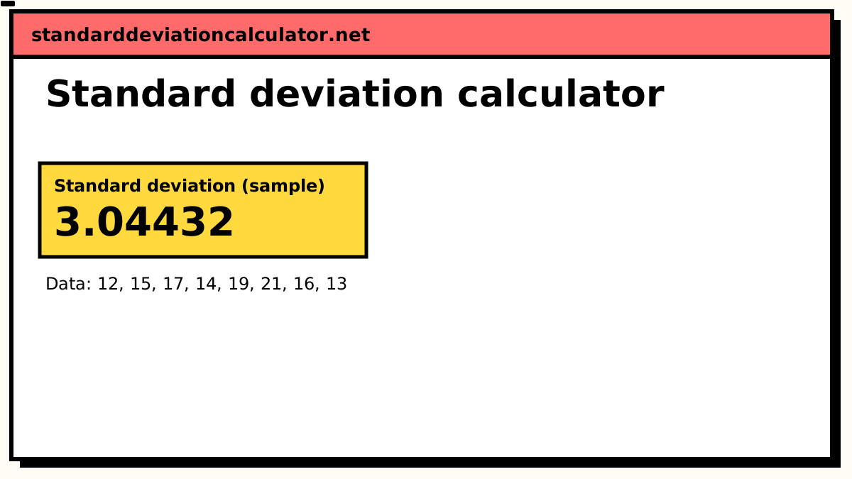
Paste the same values into the standard deviation calculator and set it to
sample. It should reproduce sd() to every displayed digit, and it lists the
count it read, so if the two disagree, a missing or non-numeric value is usually the reason,
and the count will point at it.
Related calculators
-
Standard deviation calculator
Check an R result, with every step of the working shown.
-
SD in Python
statistics, NumPy and pandas, and which one divides by n.
-
Sample vs population
Why sd() divides by n − 1, and when you should not.
-
Weighted SD calculator
The calculation R has no built-in function for.
Common questions
How do I calculate standard deviation in R?
Call sd() on a numeric vector: sd(c(12, 15, 17, 14, 19, 21, 16, 13))
returns 3.044316. It is in base R, so nothing needs installing or loading. If the vector
contains missing values, add na.rm = TRUE.
Is sd() in R the sample or population standard deviation?
Sample. sd() divides by n − 1, and so does var(). Base R has
no population version. To get the population standard deviation, compute it directly with
sqrt(mean((x - mean(x))^2)), or rescale the sample value with
sd(x) * sqrt((length(x) - 1) / length(x)).
How do I calculate variance in R?
var(x). It is the sample variance (n − 1 denominator) and
sd(x) is exactly its square root. For the population variance use
mean((x - mean(x))^2).
Why does sd() return NA in R?
Two causes. If the vector contains an NA, sd() returns
NA unless you pass na.rm = TRUE. If the vector has only one
value, sd() also returns NA, because dividing by n − 1 means
dividing by zero, and that is correct, since one observation has no spread to measure.
How do I calculate standard deviation by group in R?
Three ways, all giving the same numbers. Base R:
tapply(df$value, df$group, sd) or
aggregate(value ~ group, data = df, FUN = sd). With dplyr:
df %>% group_by(group) %>% summarise(sd = sd(value)).
How do I calculate a weighted standard deviation in R?
There is no base function. Either write one (compute the weighted mean, then
sqrt(sum(w * (x - m)^2) / (sum(w) - 1))) or install Hmisc and call
sqrt(Hmisc::wtd.var(x, w)), which uses that same frequency-weight
denominator by default.
How do I find standard deviation in RStudio?
RStudio runs R, so the commands are the same: type sd(x) in the console for the sample standard deviation of a vector x, or sd(df$column) for a data frame column.