Negative binomial distribution calculator
Enter the number of successes r you are waiting for and the success probability p, then choose whether X counts failures or trials. The calculator gives the probability of exactly, at most or at least k, with the working.
A whole number, 1 or more.
Between 0 and 1. Gives the smallest k with P(X ≤ k) ≥ p.
Each bar is P(X = k). Solid bars are the values included in the answer.
Probability table
| k | P(X = k) | P(X ≤ k) | P(X ≥ k) |
|---|---|---|---|
| 0 | 0.064 | 0.064 | 1 |
| 1 | 0.1152 | 0.1792 | 0.936 |
| 2 | 0.13824 | 0.31744 | 0.8208 |
| 3 | 0.13824 | 0.45568 | 0.68256 |
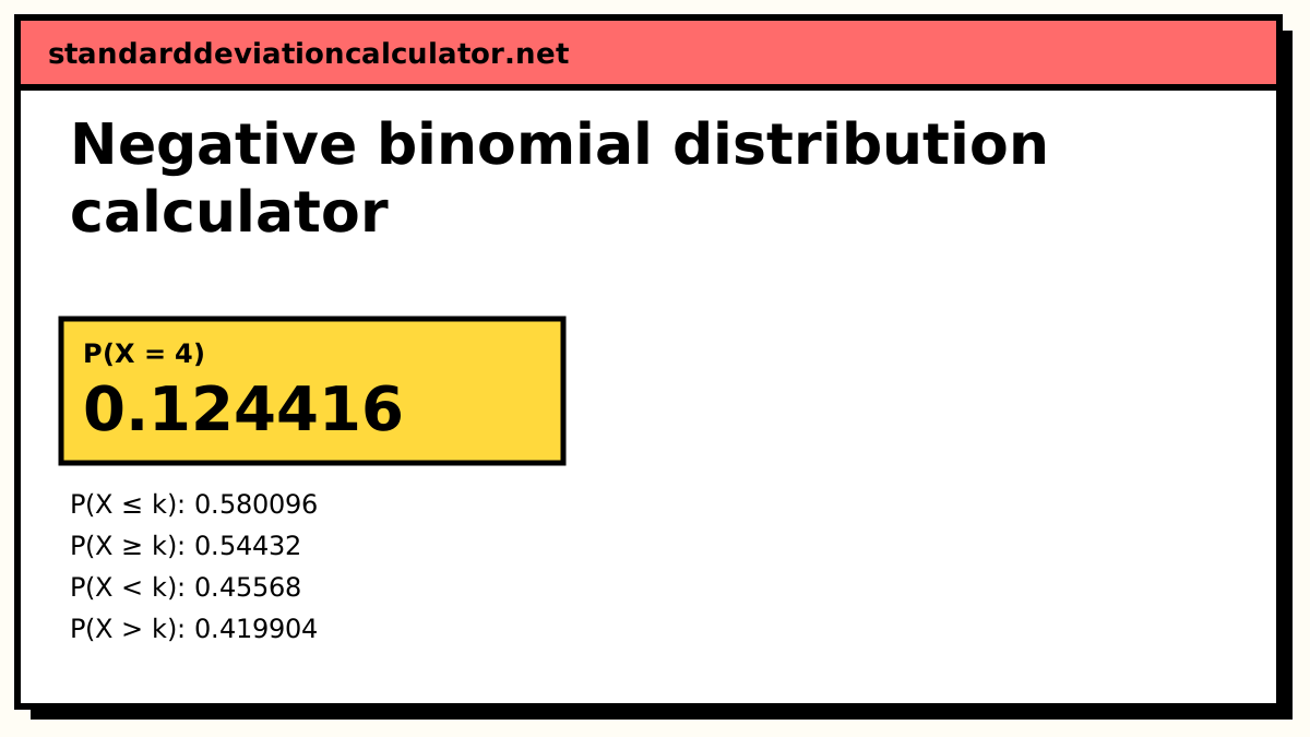
| 4 | 0.124416 | 0.580096 | 0.54432 |
| 5 | 0.104509 | 0.684605 | 0.419904 |
| 6 | 0.0836076 | 0.768213 | 0.315395 |
| 7 | 0.0644973 | 0.83271 | 0.231787 |
| 8 | 0.0483729 | 0.881083 | 0.16729 |
| 9 | 0.0354735 | 0.916557 | 0.118917 |
| 10 | 0.0255409 | 0.942098 | 0.0834433 |
| 11 | 0.0181108 | 0.960208 | 0.0579024 |
| 12 | 0.0126776 | 0.972886 | 0.0397916 |
| 13 | 0.00877679 | 0.981663 | 0.027114 |
| 14 | 0.00601837 | 0.987681 | 0.0183372 |
| 15 | 0.00409249 | 0.991774 | 0.0123188 |
| 16 | 0.00276243 | 0.994536 | 0.00822636 |
| 17 | 0.00185245 | 0.996389 | 0.00546393 |
| 18 | 0.00123497 | 0.997623 | 0.00361147 |
| 19 | 0.000818979 | 0.998442 | 0.0023765 |
| 20 | 0.000540526 | 0.998983 | 0.00155752 |
| 21 | 0.000355203 | 0.999338 | 0.001017 |
| 22 | 0.000232497 | 0.999571 | 0.000661794 |
Show the working, step by step
Probability of exactly k:
P(X = k) = C(k + r − 1, k) pr (1 − p)k P(X = 4) = C(6, 4) × 0.43 × 0.64 = 15 × 0.064 × 0.1296 = 0.124416
The formulas
Y = failures before the r-th success (k = 0, 1, 2, …):
P(Y = k) = C(k + r − 1, k) pr (1 − p)k mean = r(1 − p)/p variance = r(1 − p)/p²
X = trials up to and including the r-th success (k = r, r + 1, …):
P(X = k) = C(k − 1, r − 1) pr (1 − p)k−r mean = r/p variance = r(1 − p)/p²
The binomial coefficient counts where the first r − 1 successes can fall; the last trial must be the r-th success.
Worked example
A basketball player makes 40% of free throws. She keeps shooting until she has made 3. What is the probability that she misses exactly 4 times along the way?
P(Y = 4) = C(6, 4) × 0.4³ × 0.6⁴ = 15 × 0.064 × 0.1296 = 0.124416
Four misses means 7 shots in total, so in the trials convention the same answer is P(X = 7) = C(6, 2) × 0.4³ × 0.6⁴ = 0.124416. The cumulative probability of at most 4 misses adds the terms for 0 to 4 misses:
P(Y ≤ 4) = 0.064 + 0.1152 + 0.13824 + 0.13824 + 0.124416 = 0.580096
On average she misses 3 × 0.6/0.4 = 4.5 times (7.5 shots in total), with variance 3 × 0.6/0.16 = 11.25 and standard deviation 3.3541. The mode is a tie: (r − 1)(1 − p)/p = 3 is a whole number, so 2 and 3 misses are equally likely, each with probability 0.13824.
Reading the result
The chart is skewed right: a long run of misses is unlikely but possible, and the tail goes on without limit. The solid bars are the values counted in your answer. The median here is 4 misses, because P(Y ≤ 3) = 0.45568 and P(Y ≤ 4) = 0.580096 straddle one half.
Where it is used
Besides waiting-time questions (how many sales calls until the third sale, how many patients to screen before enrolling r who qualify), the negative binomial is the standard model for count data that vary more than a Poisson allows. In ecology, epidemiology and insurance the variance of counts is often several times the mean; the negative binomial's extra parameter absorbs that clustering, where a Poisson model would understate the uncertainty.
Common mistakes
- Mixing the conventions. If your answer is off by exactly r in the mean, you have counted failures where the question counts trials, or the reverse.
- Using C(k, r) instead of C(k − 1, r − 1). The last trial is fixed as a success, so only the earlier trials are arranged.
- Confusing it with the binomial. The binomial fixes the trials and counts successes; the negative binomial fixes the successes and counts trials.
Common questions
What does the negative binomial distribution count?
How long it takes to reach a fixed number of successes r in independent trials with success probability p. It is counted either as the number of failures before the r-th success (0, 1, 2, …) or as the total number of trials (r, r + 1, …). The geometric distribution is the special case r = 1.
Which convention does my software use?
R's dnbinom(x, size = r, prob = p), SciPy's nbinom and Excel's NEGBINOM.DIST all count failures. Many textbooks and exam boards count trials. Convert with trials = failures + r. The variance r(1 − p)/p² is the same in both.
How is the cumulative probability calculated?
By adding the terms, or through the identity P(Y ≤ k) = Ip(r, k + 1), the regularised incomplete beta function, which is what the calculator uses. Equivalently, having at most k failures before the r-th success means at least r successes in the first r + k trials, a binomial tail.
Why is it used for overdispersed counts?
Count data whose variance is larger than the mean cannot be Poisson, which forces them to be equal. The negative binomial has variance mean + mean²/r, so it fits bunched counts such as insurance claims, hospital visits or species abundance. In that role r need not be a whole number, but this calculator keeps r whole, as in the trials interpretation.
Related calculators
-
Geometric distribution
The special case r = 1: waiting for the first success.
-
Binomial distribution
Successes in a fixed number of trials, the mirror question.
-
Poisson distribution
Counts with variance equal to the mean.