Statistics
Bayes' theorem calculator
Update a prior probability with new evidence. Enter a prevalence, the test's sensitivity and its false-positive rate to see how likely a positive result is to be right, counted out for 10,000 people. Or switch to the general form for several competing hypotheses.
Decimal, fraction or percentage.
Equal to 1 − specificity.
| Per 10,000 people | Test positive | Test negative | Total |
|---|---|---|---|
| Have the condition | 90 | 10 | 100 |
| Do not have it | 891 | 9,009 | 9,900 |
| Total | 981 | 9,019 | 10,000 |
Everyone who tests positive (per 10,000 people):
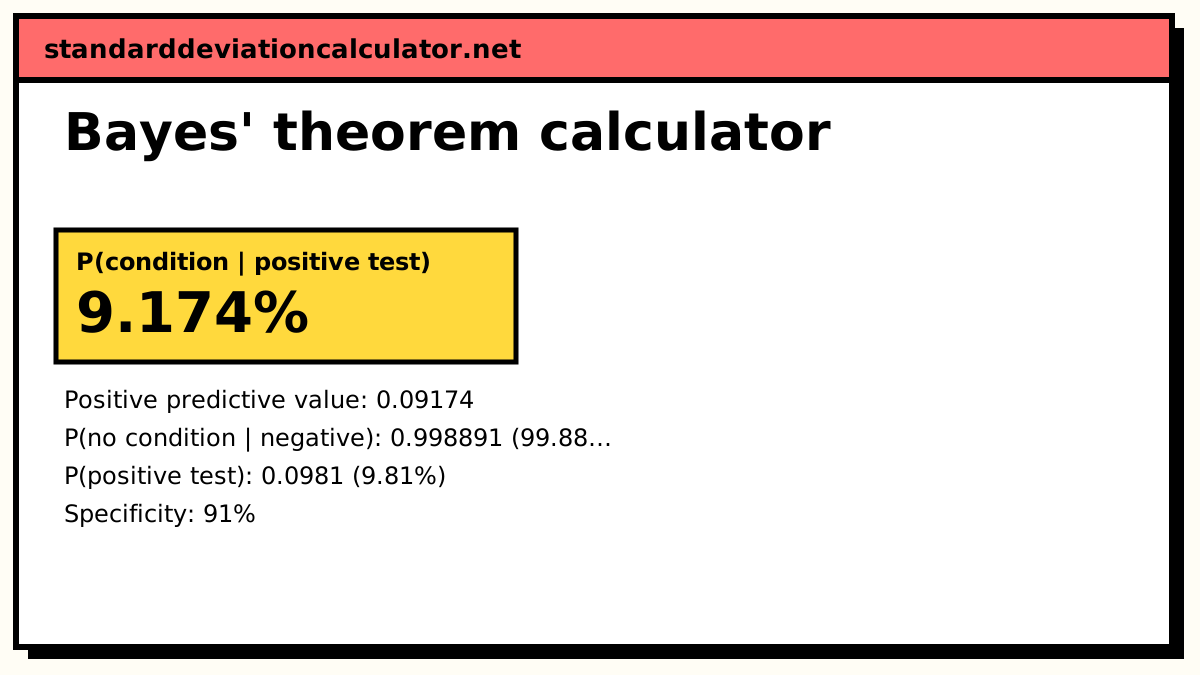
Have the condition (true positives): 90 (9.17%) Do not have it (false positives): 891 (90.8%)
Show the working, step by step
Picture 10,000 people. The prior says how many have the condition.
1% of 10,000 = 100 have it; 9,900 do not
The sensitivity finds most of those who have it.
90% of 100 = 90 true positives
The false-positive rate flags some of the much larger healthy group.
9% of 9,900 = 891 false positives
Of everyone who tests positive, the share who really have the condition:
90 ÷ (90 + 891) = 90 ÷ 981 = 9.174%
The same thing written as Bayes' theorem:
P(C|+) = P(+|C)P(C) ÷ [P(+|C)P(C) + P(+|C′)P(C′)] = 0.9 × 0.01 ÷ (0.9 × 0.01 + 0.09 × 0.99) = 0.009 ÷ 0.0981 = 0.0917431
Most positive results are false alarms here, because the condition is rare: the 9,900 people without it produce more false positives than the 100 with it produce true ones. A second, independent test is the usual next step.
The formula
P(H|E) = P(E|H) P(H) ÷ P(E)
P(E) = Σ P(E|Hᵢ) P(Hᵢ)
P(H) is the prior, P(E|H) the likelihood of the evidence if H is true, and P(H|E) the posterior. The denominator, the total probability of the evidence, adds up the ways the evidence can arise under every hypothesis. For a diagnostic test with two hypotheses (condition or not), it becomes
P(C|+) = sensitivity × prior ÷ [sensitivity × prior + false-positive rate × (1 − prior)]
A worked example: the medical test
The default: a condition affects 1% of people. The test detects 90% of cases (sensitivity) and wrongly flags 9% of healthy people (false-positive rate). Someone tests positive. How likely is it that they have the condition?
| Per 10,000 people | Test positive | Test negative | Total |
|---|---|---|---|
| Have the condition | 90 | 10 | 100 |
| Do not have it | 891 | 9,009 | 9,900 |
| Total | 981 | 9,019 | 10,000 |
Of the 981 people who test positive, 90 have the condition: 90 ÷ 981 = 9.17%. By the formula, 0.9 × 0.01 ÷ (0.9 × 0.01 + 0.09 × 0.99) = 0.009 ÷ 0.0981 = 0.0917. A negative result, by contrast, is very reassuring: 9,009 of the 9,019 negatives are truly clear, 99.89%.
Counting people rather than multiplying probabilities is called the natural-frequency method. Research by Gerd Gigerenzer and Ulrich Hoffrage found that far more people, doctors included, solve problems like this correctly when the information is given as counts rather than percentages, which is why the calculator shows the table.
A worked example: several hypotheses
The general-form default is a textbook factory problem. Machines A, B and C make 25%, 35% and 40% of the output, and 5%, 4% and 2% of their items are defective. An item chosen at random is defective. Which machine most likely made it?
- Prior × likelihood: A 0.25 × 0.05 = 0.0125; B 0.35 × 0.04 = 0.014; C 0.40 × 0.02 = 0.008.
- Total probability of a defective item: 0.0125 + 0.014 + 0.008 = 0.0345.
- Posteriors: A 0.0125 ÷ 0.0345 = 25/69 = 0.3623; B 28/69 = 0.4058; C 16/69 = 0.2319.
Machine C makes the most items but has the lowest defect rate, so a defective item most likely came from B.
Common mistakes
- Ignoring the base rate. Reading the 90% sensitivity as the chance a positive is right. That is P(+|C), not P(C|+).
- Using specificity where the false-positive rate is needed. Enter 9%, not 91%, in the false-positive field.
- Priors that do not cover every case. In the general form the hypotheses must be exhaustive and mutually exclusive for the posteriors to mean what they say.
Common questions
What is Bayes' theorem?
A rule for reversing a conditional probability: P(A|B) = P(B|A) P(A) ÷ P(B). In words, the probability of a cause given the evidence equals the probability of the evidence given the cause, times the prior probability of the cause, divided by the overall probability of the evidence. It is how a prior belief is updated when new information arrives.
Why is the chance of having the disease so low after a positive test?
Because the condition is rare. With 1% prevalence, 10,000 people include 100 who have it and 9,900 who do not. A 90% sensitive test finds 90 of the 100, but a 9% false-positive rate also flags 891 of the 9,900. Of the 981 positives, only 90 are real: 9.2%. The test is informative (it raised the probability from 1% to 9.2%) but a single positive is far from a diagnosis. This is the base-rate fallacy.
What happens after a second positive test?
Use the first posterior as the new prior. If a second, independent test with the same accuracy is also positive, the prior is 0.0917 and the posterior becomes 0.9 × 0.0917 ÷ (0.9 × 0.0917 + 0.09 × 0.9083) = 0.503, about 50%. Enter 9.174% as the prior to check. The assumption that the two tests' errors are independent matters: repeating the same test on the same sample often is not.
What are sensitivity, specificity and the false-positive rate?
Sensitivity is P(positive | condition), the share of true cases the test catches. Specificity is P(negative | no condition), the share of healthy people it correctly clears. The false-positive rate is 1 − specificity. A test with 91% specificity has a 9% false-positive rate.
Do the priors in the general form have to add up to 1?
They should, because the hypotheses should cover every possibility with no overlap. If they do not, the calculator rescales them to add to 1 and says so. The likelihoods do not need to add to anything: each is the probability of the same evidence under a different hypothesis.
Related calculators
-
Conditional probability
P(A|B) from probabilities or from a table of counts.
-
Probability calculator
And, or, not and at-least-one probabilities.
-
Logistic regression
Model the probability of an outcome from several predictors.
-
Binomial distribution
Probabilities for a count of successes in n trials.