Statistics
Logistic regression calculator
Enter a 0/1 outcome and one to three predictors to fit a logistic regression. The calculator finds the maximum-likelihood coefficients, tests each one, converts them to odds ratios and predicts the probability of y = 1 for values you choose.
Fill in one value per predictor in use.
Dots at 0 and 1 are the observed outcomes; the curve is the fitted probability, and the yellow point is your prediction.
| Term | Coefficient b | Std. error | Wald z | p-value | Odds ratio eᵇ | 95% CI for OR |
|---|---|---|---|---|---|---|
| Intercept | −4.07771 | 1.761 | −2.3156 | 0.02058 | — | — |
| x1 | 1.50465 | 0.62872 | 2.3932 | 0.0167 | 4.5026 | 1.313 to 15.44 |
Show the working, step by step
The model: the log-odds of y = 1 is linear in the predictors.
ln(p ÷ (1 − p)) = b₀ + b₁x₁ + …, p = 1 ÷ (1 + e^−(b₀ + b₁x₁ + …))
Maximise the log-likelihood ℓ = Σ[y ln p + (1 − y) ln(1 − p)] by Newton–Raphson (IRLS), starting from the intercept-only model. It converged in 7 iterations.
iteration 0: ℓ = −13.862944 iteration 1: ℓ = −8.5602871 iteration 2: ℓ = −8.0679669 iteration 3: ℓ = −8.0302676 iteration 4: ℓ = −8.0298785 iteration 5: ℓ = −8.0298785 iteration 6: ℓ = −8.0298785 iteration 7: ℓ = −8.0298785
Standard errors are the square roots of the diagonal of the inverse information matrix (X′WX)⁻¹, with W = p(1 − p). Each Wald z is b ÷ SE.
Intercept: z = −4.07771 ÷ 1.761 = −2.3156, p = 0.02058 x1: z = 1.50465 ÷ 0.62872 = 2.3932, p = 0.0167
Compare with the intercept-only model.
ℓ₀ = n₁ ln(n₁/n) + n₀ ln(n₀/n) = −13.8629 LR χ² = 2(ℓ − ℓ₀) = 11.666, McFadden R² = 1 − ℓ/ℓ₀ = 0.42077
Predicted probability: compute the log-odds η, then p = 1 ÷ (1 + e^−η).
η = −4.07771 + 1.50465 × 2 = −1.06842 p = 0.2557
Each odds ratio is the factor by which the odds of y = 1 multiply for a one-unit rise in that predictor, holding the others fixed. McFadden values of 0.2 to 0.4 already indicate a good fit; they run much lower than an OLS R².
The model
ln( p ÷ (1 − p) ) = b₀ + b₁x₁ + b₂x₂ + …
p = 1 ÷ (1 + e^−(b₀ + b₁x₁ + b₂x₂ + …))
The left side of the first equation is the log-odds, or logit, of y = 1. It can take any value, so it can be modelled as a straight line in the predictors, while p itself stays between 0 and 1. There is no closed-form solution: the coefficients are the values that maximise the log-likelihood
ℓ = Σ [ yᵢ ln pᵢ + (1 − yᵢ) ln(1 − pᵢ) ]
found here by Newton–Raphson, which for this model is the same as iteratively reweighted least squares. Each step solves a weighted least-squares problem with weights p(1 − p) and the inverse of the final weighted matrix gives the standard errors.
A worked example
The default data are the widely used example of 20 students, the hours each spent studying and whether they passed the exam (1) or not (0). The fit converges in a few iterations to
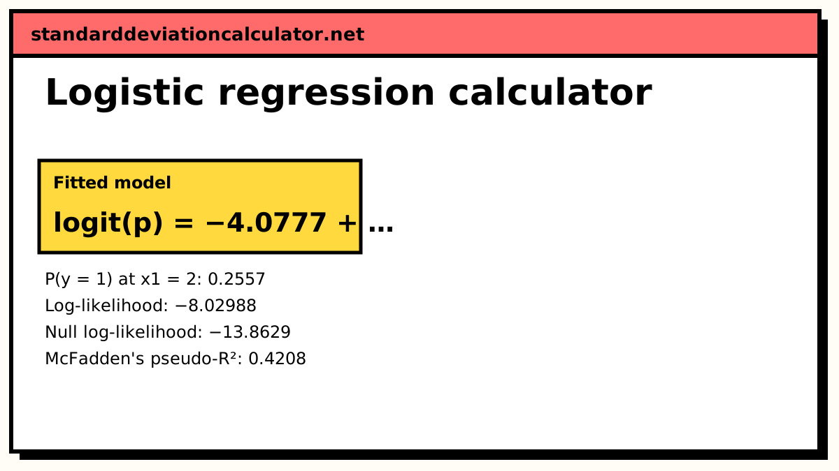
logit(p) = −4.0777 + 1.5046 × hours
| Term | b | SE | Wald z | p | Odds ratio |
|---|---|---|---|---|---|
| Intercept | −4.0777 | 1.7610 | −2.316 | 0.0206 | — |
| Hours | 1.5046 | 0.6287 | 2.393 | 0.0167 | 4.50 |
The log-likelihood rises from ℓ₀ = 20 ln 0.5 = −13.863 for the intercept-only model to ℓ = −8.030, a likelihood-ratio χ² of 11.67 on 1 degree of freedom (p = 0.0006). McFadden's pseudo-R² is 1 − 8.030 ÷ 13.863 = 0.42.
For a student who studies 2 hours, the log-odds are −4.0777 + 1.5046 × 2 = −1.068, so p = 1 ÷ (1 + e1.068) = 0.256. At 4 hours the probability is 0.874. The 50% point is where the log-odds are zero: 4.0777 ÷ 1.5046 = 2.71 hours.
Entering data
- Put the outcome in the first column as 0 or 1 only. Recode yes/no or categories before entering them.
- Use x1, then x2 and x3 as needed. A column left completely blank is ignored; a row with a blank in a column that is in use is skipped.
- A categorical predictor with two levels can be entered as 0/1. One with more levels needs one 0/1 column per level except a reference level.
- To predict, fill in one value for each predictor in use in the fields under the table.
Common problems
- Separation. When a predictor splits the 0s and 1s perfectly, the estimates are infinite. The calculator reports this rather than a misleading number.
- Too few events. A common guide is at least 10 events (the rarer of the 0s and 1s) per predictor. With fewer, estimates are biased away from zero.
- Reading coefficients as probabilities. b is a change in log-odds. The change in probability for a one-unit step depends on where you start on the S-shaped curve.
Common questions
When should I use logistic regression instead of linear regression?
When the outcome is binary: pass or fail, bought or did not, disease or no disease. A straight line fitted to 0s and 1s predicts probabilities below 0 and above 1 and has errors that cannot be normal. Logistic regression models the log-odds instead, so every prediction is a probability between 0 and 1.
How do I interpret the odds ratio?
eb is the factor by which the odds of y = 1 multiply for each one-unit increase in that predictor, with the others held constant. In the default example the odds ratio for hours of study is 4.50: each extra hour multiplies the odds of passing by about 4.5. An odds ratio of 1 means no effect, and one below 1 means the odds fall as the predictor rises.
What is McFadden's pseudo-R²?
1 − ℓ ÷ ℓ₀, where ℓ is the log-likelihood of the fitted model and ℓ₀ that of a model with only an intercept. It is not the share of variance explained, and it runs much lower than an ordinary R²: values from 0.2 to 0.4 are usually read as a good fit. The example gives 0.42.
What does 'the model did not converge' mean?
Usually that a predictor separates the outcomes perfectly or almost perfectly: for example, everyone who studied more than 3 hours passed and everyone below failed. The likelihood then keeps increasing as the slope grows, so the maximum-likelihood estimate is infinite. The calculator stops rather than report a huge coefficient with a meaningless standard error. Options are more data, dropping or combining the separating predictor, or penalised (Firth) logistic regression.
Why are Wald p-values different from the likelihood-ratio test?
They are two approximations to the same question. The Wald test uses the coefficient and its standard error; the likelihood-ratio test compares log-likelihoods of models with and without the predictor. They agree in large samples. In small samples, or with large coefficients, the likelihood-ratio test is more reliable.
Related calculators
-
Multiple regression
Least-squares regression for a continuous outcome with several predictors.
-
Linear regression calculator
Straight-line fit of one y on one x.
-
Probability calculator
Rules for combining the probabilities of events.
-
Chi-square calculator
Test association between two categorical variables.