Exponential regression calculator
Fit an exponential growth or decay curve to paired data. The calculator takes logs, fits a straight line, and transforms back to give y = a·e^(bx), the equivalent y = a·b^x, the percentage growth rate and a prediction.
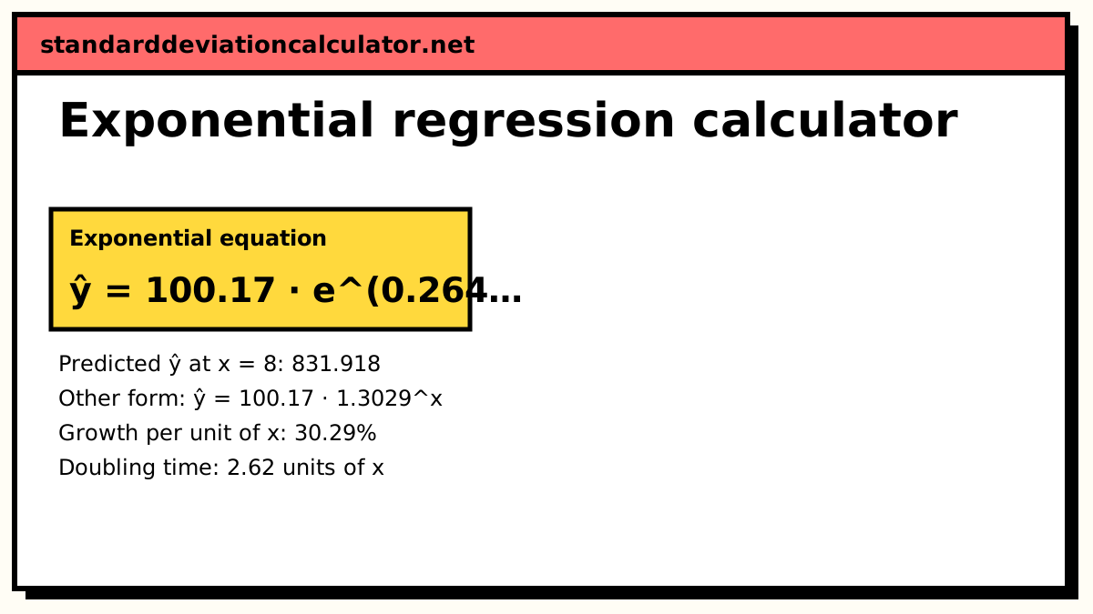
━ Data ━ ŷ = 100.17 · e^(0.2646x)
| x | y | ln y | ŷ | y − ŷ |
|---|---|---|---|---|
| 0 | 100 | 4.60517 | 100.174 | −0.17431 |
| 1 | 130 | 4.86753 | 130.518 | −0.51844 |
| 2 | 172 | 5.14749 | 170.054 | 1.9458 |
| 3 | 220 | 5.39363 | 221.566 | −1.5659 |
| 4 | 290 | 5.66988 | 288.681 | 1.3189 |
| 5 | 375 | 5.92693 | 376.126 | −1.1264 |
| 6 | 490 | 6.19441 | 490.06 | −0.060041 |
Show the working, step by step
Take the natural log of each y. Since ln(a·e^(bx)) = ln a + bx, a straight line through (x, ln y) gives the curve.
mean of x = 3, mean of ln y = 5.40072
Least-squares slope and intercept of ln y on x.
b = Σ(x − x̄)(ln y − mean) ÷ Σ(x − x̄)² = 7.40888 ÷ 28 = 0.264603 ln a = 5.40072 − 0.264603 × 3 = 4.60691
Transform back.
a = e^(4.60691) = 100.174 growth factor = e^b = e^(0.264603) = 1.30291 ŷ = 100.17 · e^(0.2646x) ŷ = 100.17 · 1.3029^x
How well the line fits on the log scale.
R² = 0.999884; t for b = 207.16 with 5 df, p < 0.0001
Prediction at x = 8.
ŷ = 100.174 × e^(0.264603 × 8) = 831.918
On the log scale this is a very close fit. Because the fit minimises squared errors in ln y, not in y, it weights small y values more heavily than a direct non-linear fit would; the R² on y shows how it does on the original scale.
The method
y = a·e^(bx) ⇒ ln y = ln a + bx b = Σ(x − x̄)(ln y − mean ln y) ÷ Σ(x − x̄)² ln a = mean ln y − b·x̄, growth factor = e^b
Taking the natural log turns the curve into a straight line in x, so ordinary least squares applies. The slope of that line is b, and its intercept is ln a.
A worked example
The default data are seven counts of a growing population at x = 0 to 6: y = 100, 130, 172, 220, 290, 375, 490. Each value is roughly 1.3 times the one before, which is the mark of exponential growth.
- Take logs: ln 100 = 4.605, ln 130 = 4.868, and so on. The mean of ln y is 5.40072 and x̄ = 3.
- The slope of ln y on x is b = 7.40888 ÷ 28 = 0.264603.
- The intercept is ln a = 5.40072 − 0.264603 × 3 = 4.60691, so a = e^4.60691 = 100.17.
- The growth factor is e^0.264603 = 1.3029.
ŷ = 100.17 · e^(0.2646x) = 100.17 · 1.3029^x
The population grows by about 30.3% per step in x and doubles every ln 2 ÷ 0.2646 = 2.62 steps. The straight line through (x, ln y) has R² = 0.99988. The default prediction at x = 8 is 100.17 × e^(0.2646 × 8) = 831.9, which the calculator flags because 8 lies beyond the last data point.
How to read the result
A positive b means growth and a negative b means decay. The percentage change per unit of x is (e^b − 1) × 100%, not b × 100%. The two are close only when b is small. For b = 0.2646 the true rate is 30.3%, not 26.5%. a is the fitted value at x = 0. If your x values are years such as 2019 to 2025, a is the value in year 0, which is meaningless. Subtract the first year from x first. Check the chart: if the points bend away from the curve at the ends, growth is slowing, and a logistic or polynomial model may fit better.
Checking that the model suits the data
The quickest check is to plot ln y against x. If those points fall close to a straight line, the exponential model is right. If they curve, it is not. The residual column in the table gives the same information on the original scale. A run of positive residuals in the middle and negative ones at the ends means the growth is slowing. A steady ratio between successive y values, as in the default data, is the pattern to look for.
Common mistakes
- Using log base 10 and then e. If you take log₁₀ y by hand, the slope is log₁₀ of the growth factor, not b. Stick to one base.
- Reading b as a percentage. The growth rate is e^b − 1.
- Including zero or negative y values. They cannot be logged, so the fit is impossible.
- Long-range extrapolation. Real growth rarely stays exponential for long.
Common questions
What is the difference between y = a·e^(bx) and y = a·b^x?
They are the same curve written two ways. The growth factor per unit of x is e^b in the first form and the base in the second, so the base equals e^b. In the default example b = 0.2646 and e^0.2646 = 1.3029: y grows by 30.29% for each step in x. Calculators such as the TI-84 report the a·b^x form.
Why must every y be positive?
The fit works on ln y, and the logarithm of zero or a negative number is undefined. An exponential curve a·e^(bx) with a > 0 is always positive anyway. If your data include zeros, consider adding a constant before fitting, or a different model.
Why are there two R² values?
Least squares is done on ln y, so the natural R² is the one for the straight line through (x, ln y). The calculator also reports 1 − SSE/SST on the original y scale using the fitted curve, which tells you how close the curve comes to the raw values. For well-behaved growth data the two are close, as in the default (0.99988 and 0.99992).
Is this the same answer as a non-linear least-squares fit?
Close but not identical. Fitting on the log scale minimises relative (percentage) errors, which gives small y values more weight. A direct non-linear fit minimises errors in y itself and weights the large values more. The log-linear fit is the standard textbook and graphing-calculator method.
How do I get the doubling time or half-life?
Doubling time = ln 2 ÷ b when b is positive; half-life = ln 2 ÷ |b| when b is negative. The calculator shows whichever applies. For the default data, ln 2 ÷ 0.2646 = 2.62 units of x.
Related calculators
-
Linear regression calculator
The straight-line fit that exponential regression uses on ln y.
-
Polynomial regression calculator
Curved fits of degree 1 to 6 when growth is not exponential.
-
Compound interest calculator
Exponential growth of money at a fixed rate.