Polynomial regression calculator
Fit a polynomial curve of your chosen degree to paired data. The calculator gives the equation, R² and adjusted R², draws the curve, and fits every other degree too so you can pick the right one.
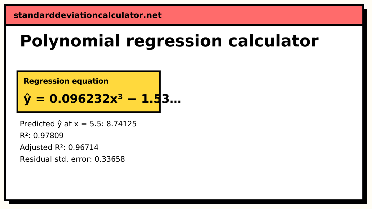
━ Data ━ ŷ = 0.096232x³ − 1.5371x² + 6.697x + 2.3933
| Term | Coefficient |
|---|---|
| a (x³) | 0.096231546 |
| b (x²) | −1.5370629 |
| c (x) | 6.6970085 |
| d (Constant) | 2.3933333 |
| x | y | ŷ | Residual y − ŷ |
|---|---|---|---|
| 1 | 7.8 | 7.64951 | 0.15049 |
| 2 | 10 | 10.409 | −0.40895 |
| 3 | 11.5 | 11.249 | 0.25096 |
| 4 | 10.9 | 10.7472 | 0.15282 |
| 5 | 9.2 | 9.48075 | −0.28075 |
| 6 | 8.4 | 8.02713 | 0.37287 |
| 7 | 6.7 | 6.96373 | −0.26373 |
| 8 | 6.7 | 6.86793 | −0.16793 |
| 9 | 8.6 | 8.31711 | 0.28289 |
| 10 | 11.8 | 11.8887 | −0.088671 |
| Degree | R² | Adjusted R² | Residual std. error |
|---|---|---|---|
| 1 | 0.012252 | -0.11122 | 1.9572 |
| 2 | 0.056099 | -0.21359 | 2.0453 |
| 3 | 0.97809 | 0.96714 | 0.33658 |
| 4 | 0.97825 | 0.96086 | 0.36733 |
| 5 | 0.9844 | 0.96491 | 0.34779 |
| 6 | 0.98445 | 0.95336 | 0.40097 |
Show the working, step by step
Set up the model ŷ = ax³ + bx² + cx + d and the design matrix with columns 1, x, x², x³ for the 10 points.
Solve the least-squares problem (minimise Σ(y − ŷ)²). The calculator centres and scales x first and uses a QR decomposition, which gives the same answer as the normal equations with far less rounding error.
ŷ = 0.096232x³ − 1.5371x² + 6.697x + 2.3933
Split the variation in y.
SST = Σ(y − ȳ)² = 31.024 SSE = Σ(y − ŷ)² = 0.679711 SSR = SST − SSE = 30.3443
Coefficient of determination and its adjusted form.
R² = 1 − SSE ÷ SST = 1 − 0.679711 ÷ 31.024 = 0.978091 adjusted R² = 1 − (1 − R²)(n − 1) ÷ (n − 3 − 1) = 1 − 0.0219092 × 9 ÷ 6 = 0.967136
Overall F-test of H₀: every non-constant coefficient is zero.
F = (SSR ÷ 3) ÷ (SSE ÷ 6) = 89.286, p < 0.0001
Prediction at x = 5.5: substitute into the equation.
ŷ(5.5) = 8.74125
A very close fit: the curve explains 97.81% of the variation in y. Adding degrees always raises R²; compare adjusted R² when choosing the degree.
The model
ŷ = b₀ + b₁x + b₂x² + … + b_d x^d R² = 1 − SSE ÷ SST, adjusted R² = 1 − (1 − R²)(n − 1) ÷ (n − d − 1)
The d + 1 coefficients minimise the sum of squared residuals Σ(y − ŷ)². A degree-d fit needs at least d + 2 points and d + 1 distinct x values. The calculator centres and scales x, solves by QR decomposition, and converts the result back to powers of the original x. That keeps the answer accurate at degree 6, where the textbook normal equations lose most of their digits.
A worked example
The default data are ten readings at x = 1 to 10: y = 7.8, 10, 11.5, 10.9, 9.2, 8.4, 6.7, 6.7, 8.6, 11.8. The values rise, fall and rise again. Fitting each degree gives:
| Degree | R² | Adjusted R² | Residual SE |
|---|---|---|---|
| 1 | 0.0123 | −0.1112 | 1.957 |
| 2 | 0.0561 | −0.2136 | 2.045 |
| 3 | 0.9781 | 0.9671 | 0.337 |
| 4 | 0.9783 | 0.9609 | 0.367 |
| 5 | 0.9844 | 0.9649 | 0.348 |
| 6 | 0.9845 | 0.9534 | 0.401 |
R² climbs at every step, but adjusted R² peaks at degree 3 and the residual standard error is smallest there. The degrees above 3 buy almost nothing and pay for it in degrees of freedom. The cubic is
ŷ = 0.096232x³ − 1.5371x² + 6.697x + 2.3933
with R² = 0.97809, adjusted R² = 0.96714 and F(3, 6) = 89.29 (p below 0.0001). The default prediction at x = 5.5 is ŷ = 8.74.
How to interpret the output
The overall F-test asks whether the polynomial explains more than a flat line at ȳ. It does not say the degree is right. Use the comparison table for that. The coefficients of a high-degree polynomial are hard to interpret one at a time, because x, x², x³ and so on are strongly correlated. Treat the curve as a whole and use it for fitted values and predictions inside the data range. The residual table shows where the curve misses; a run of residuals with the same sign means the degree is too low.
Entering your data
Type or paste one (x, y) pair per row. Use Add row for more rows. Rows with a blank or non-numeric cell are skipped, and the calculator tells you how many. Repeated x values are fine and common in experiments, but you need at least d + 1 different x values for a degree-d fit. Change the degree with the menu and the equation, chart and statistics update, while the comparison table stays the same.
Common mistakes
- Choosing the degree with the highest R². That is always the highest degree. Use adjusted R², a hold-out set or the residuals.
- Extrapolating a high-degree fit. Beyond the data, a degree-5 or 6 polynomial can shoot off in any direction.
- Fitting as many coefficients as points. With n points and degree n − 1 the curve is exact and tells you nothing about the pattern.
- Rounding coefficients. Small high-power coefficients multiply large numbers. Round only the final predictions.
Common questions
How do I choose the degree?
Start low and go up only while adjusted R² improves clearly and the residual plot loses its pattern. The table under the result fits every degree the data allow, so you can see where the gain stops. In the default data, adjusted R² jumps from −0.21 at degree 2 to 0.967 at degree 3, then drifts down. Degree 3 is the choice.
Why does R² keep going up with the degree?
Each extra term gives the curve one more way to bend towards the points, and least squares will never make the fit worse by using it. With n points a polynomial of degree n − 1 passes through all of them and R² = 1, even for pure noise. That is overfitting, and adjusted R² is there to catch it.
Can adjusted R² be negative?
Yes. It is negative when the model explains less than it costs in degrees of freedom. Here the straight line gives R² = 0.012 and adjusted R² = −0.111, which says a line tells you nothing about these data.
Is polynomial regression linear or non-linear regression?
Linear. The curve is non-linear in x, but the model is linear in its coefficients, so ordinary least squares solves it exactly with no iteration. Non-linear regression means models like y = a·e^(bx), where a coefficient sits inside a non-linear function.
Why stop at degree 6?
Above degree 5 or 6 polynomials swing wildly between and beyond the data points (Runge's phenomenon), and the coefficients become very sensitive to small changes in the data. For more flexible shapes a spline or a transformation of x is usually a better tool.
Related calculators
-
Quadratic regression calculator
The degree-2 fit, with the parabola explained step by step.
-
Cubic regression calculator
The degree-3 fit for data with two bends.
-
Multiple regression calculator
Least squares with several separate predictors.