Matthews correlation coefficient calculator
Score a classifier with the Matthews correlation coefficient. Enter the four counts from a binary confusion matrix, or paste a K × K matrix, and the calculator gives MCC with the working and the other common metrics.
One row per line; separate counts with spaces or commas.
The other scores run from 0 to 1 and can look high on imbalanced data; MCC runs from −1 to +1 and is only high when all four cells are good.
| Predicted positive | Predicted negative | Total | |
|---|---|---|---|
| Actual positive | TP = 90 | FN = 10 | 100 |
| Actual negative | FP = 20 | TN = 80 | 100 |
| Total | 110 | 90 | 200 |
Show the working, step by step
Numerator: correct products minus error products.
TP×TN − FP×FN = 90×80 − 20×10 = 7200 − 200 = 7000
Denominator: the square root of the four margins multiplied together.
√((TP+FP)(TP+FN)(TN+FP)(TN+FN)) = √(110 × 100 × 100 × 90) = √99000000 = 9949.87
Divide.
MCC = 7000 ÷ 9949.87 = 0.703526
MCC is Pearson’s correlation between the actual and predicted labels coded 0/1 (the phi coefficient). +1 is perfect prediction, 0 is no better than chance and −1 is total disagreement.
The formula
MCC = (TP × TN − FP × FN) ÷ √((TP + FP)(TP + FN)(TN + FP)(TN + FN))
TP and TN are the correct positive and negative predictions; FP and FN are the two kinds of mistake. The four brackets in the denominator are the row and column totals of the confusion matrix. MCC is Pearson's correlation coefficient between the actual and predicted labels coded as 0 and 1, which is why it runs from −1 to +1.
A worked example
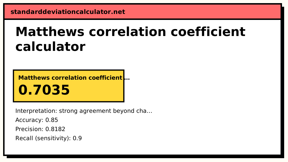
The default is a screening model tested on 100 positive and 100 negative cases. It catches 90 of the positives (TP = 90, FN = 10) and correctly clears 80 of the negatives (TN = 80, FP = 20).
numerator = 90 × 80 − 20 × 10 = 7200 − 200 = 7000 denominator = √(110 × 100 × 100 × 90) = √99,000,000 = 9949.9 MCC = 7000 ÷ 9949.9 = 0.7035
An MCC of 0.70 is strong agreement. The same model has accuracy 0.85, precision 0.818, recall 0.90 and F1 0.857. Those figures all look better than the MCC, which is typical: MCC is the stricter measure because it penalises weakness on either class.
Why MCC is harder to fool
Suppose a data set has 950 negatives and 50 positives, and a lazy model predicts negative every time. Accuracy is 95%. But TP = 0 and FP = 0, so the column of positive predictions is empty, the denominator is 0, and MCC is reported as 0: the model has learned nothing. Change it to catch 25 of the positives with 25 false alarms and MCC becomes (25 × 925 − 25 × 25) ÷ √(50 × 50 × 950 × 950) = 0.47, a fair reflection of a model that is useful but far from perfect.
Multiclass MCC
Switch to the multiclass option to paste a confusion matrix with actual classes as rows and predicted classes as columns. The default 3 × 3 matrix has 129 of 150 cases on the diagonal (accuracy 0.86); row totals 55, 50, 45 and column totals 55, 48, 47 give
MCC = (129 × 150 − Σ tₖpₖ) ÷ √((150² − Σpₖ²)(150² − Σtₖ²)) = 11810 ÷ 14956 = 0.790
Common mistakes
- Swapping FP and FN. MCC itself is unchanged, but precision and recall trade places, so the other metrics you report will be wrong.
- Transposing the multiclass matrix. MCC is unchanged by the transpose, but the row and column labels in your report will be wrong.
- Reading MCC as a percentage. 0.70 is a correlation, not 70% accuracy.
- Averaging MCC across folds with very different class balances without also reporting the spread.
Common questions
What is the Matthews correlation coefficient?
A single number that summarises how well a binary classifier's predictions agree with the true labels, using all four cells of the confusion matrix. It was introduced by the biochemist Brian Matthews in 1975 and is the same quantity as the phi coefficient for a 2×2 table.
Why use MCC instead of accuracy or F1?
Accuracy is misleading when the classes are imbalanced: a model that calls everything negative scores 95% accuracy on data that are 95% negative, yet has MCC = 0. F1 ignores true negatives entirely and changes if you swap which class is called positive. MCC is high only when the model does well on both classes, and it is symmetric in the two classes.
What is a good MCC value?
+1 is perfect, 0 is no better than random guessing and −1 is perfect disagreement. As a rough guide, above 0.7 is strong, 0.4 to 0.7 moderate and below 0.2 weak, but what counts as good depends on how hard the problem is. Compare against a baseline model on the same data.
What happens when the denominator is zero?
If a whole row or column of the confusion matrix is empty, for example the model never predicts the positive class, the formula is 0/0. The usual convention, followed by scikit-learn and by this calculator, is to report MCC = 0.
How does MCC work with more than two classes?
Gorodkin's generalisation uses the whole K × K confusion matrix: the number of correct predictions c, the total s, and the row and column totals. It reduces to the binary formula when K = 2. Its minimum is between −1 and 0 depending on the class distribution, while the maximum is still +1.
Related calculators
-
Correlation coefficient calculator
Pearson's r for two numeric variables.
-
Pearson correlation coefficient calculator
r by three methods, with a significance test.
-
Chi-square calculator
Test whether the rows and columns of a table are independent.