Statistics
Multiple regression calculator
Enter a response y and up to four predictors to fit ŷ = b₀ + b₁x₁ + … by least squares. The calculator solves the normal equations and reports each coefficient with its standard error and t-test, the fit statistics and the overall F-test.
┄ perfect fit: actual = fitted
Each dot is one row. The closer the dots hug the diagonal, the higher R² (0.9863); the vertical gap from the line is that row's residual.
| Term | Coefficient | Std. error | t | p-value | Significant at 0.05? |
|---|---|---|---|---|---|
| Intercept | 53.6 | 2.0875 | 25.677 | < 0.0001 | Yes |
| x1 | 2.35061 | 0.21849 | 10.759 | < 0.0001 | Yes |
| x2 | −0.107895 | 0.56006 | −0.19265 | 0.8527 | No |
| Source | SS | df | MS | F | p-value |
|---|---|---|---|---|---|
| Regression | 647.129 | 2 | 323.564 | 252.46 | < 0.0001 |
| Residual | 8.97146 | 7 | 1.28164 | ||
| Total | 656.1 | 9 |
Show the working, step by step
Write the model with 2 predictors and an intercept, and form the normal equations (X′X)b = X′y from the 10 rows.
10·b0 + 91·b1 + 64·b2 = 743 91·b0 + 949·b1 + 624·b2 = 7041 64·b0 + 624·b1 + 428·b2 = 4851
Solve the 3 × 3 system (here by inverting the centred cross-product matrix, which gives the same answer with less rounding).
b0 = 53.6 b1 = 2.35061 b2 = −0.107895
Split the variation in y.
SST = 656.1, SSR = 647.129, SSE = 8.97146 R² = SSR ÷ SST = 0.986326 adjusted R² = 1 − (1 − R²)(n − 1) ÷ (n − k − 1) = 1 − 0.0136739 × 9 ÷ 7 = 0.982419
Overall F-test of H₀: every slope is zero.
F = (SSR ÷ k) ÷ (SSE ÷ (n − k − 1)) = (647.129 ÷ 2) ÷ (8.97146 ÷ 7) = 252.46, p = < 0.0001
Each coefficient: t = b ÷ SE(b), with SE(b) = √(MSE × the diagonal of (X′X)⁻¹) and df = 7. Critical t at α = 0.05: ±2.3646.
Intercept: t = 53.6 ÷ 2.0875 = 25.677 x1: t = 2.35061 ÷ 0.21849 = 10.759 x2: t = −0.107895 ÷ 0.56006 = −0.19265
Each slope is the change in ŷ for a one-unit rise in that predictor with the other predictors held fixed. The model as a whole is significant at α = 0.05.
The model and the normal equations
y = β₀ + β₁x₁ + β₂x₂ + … + βₖxₖ + ε
(X′X) b = X′y ⇒ b = (X′X)⁻¹ X′y
X is the data matrix with a column of 1s for the intercept. Least squares chooses the coefficients that make the sum of squared residuals Σ(y − ŷ)² as small as possible, and setting its derivatives to zero gives the normal equations above: one equation per coefficient.
SE(bⱼ) = √(MSE × [(X′X)⁻¹]ⱼⱼ), t = bⱼ ÷ SE(bⱼ), df = n − k − 1
F = (SSR ÷ k) ÷ (SSE ÷ (n − k − 1))
A worked example
The default data are ten students' exam scores (y), weekly hours of study (x1) and nightly hours of sleep (x2). The normal equations are:
10b₀ + 91b₁ + 64b₂ = 743 91b₀ + 949b₁ + 624b₂ = 7041 64b₀ + 624b₁ + 428b₂ = 4851
Solving them gives the fitted equation
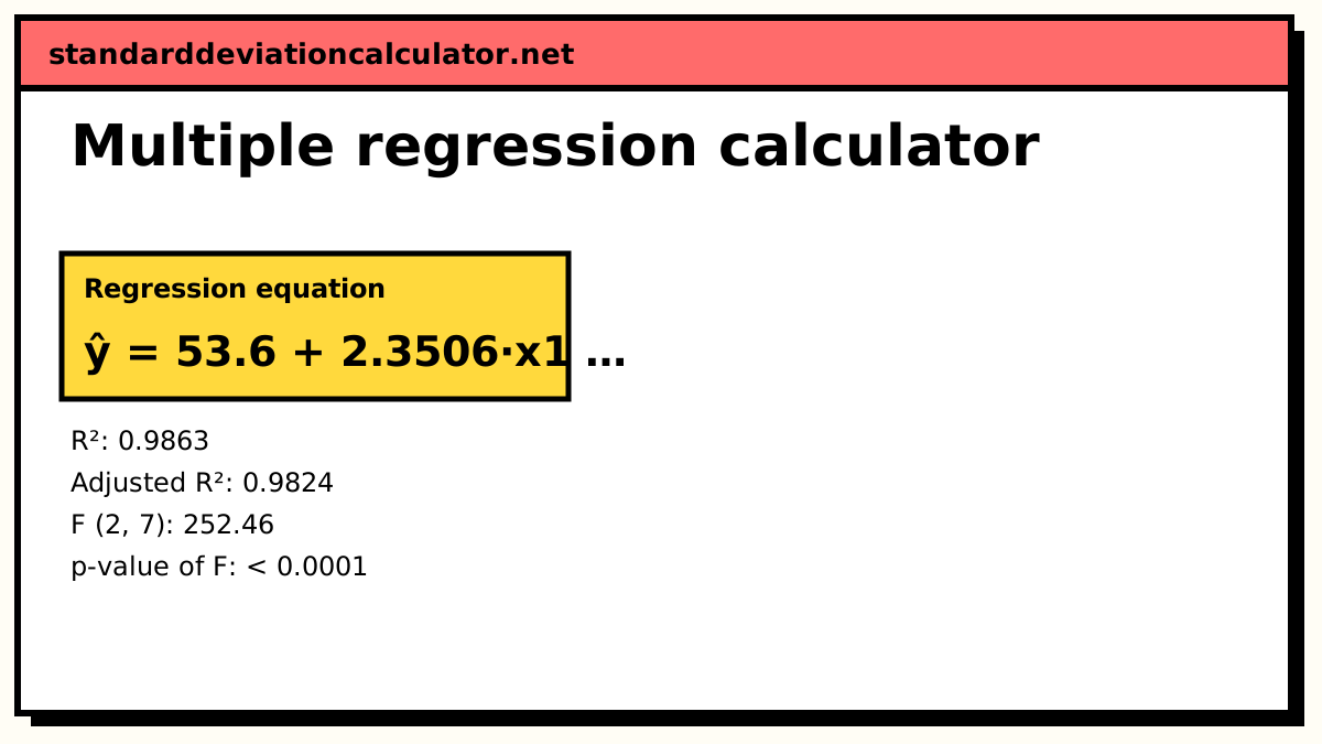
ŷ = 53.6 + 2.3506·x1 − 0.1079·x2
| Term | Coefficient | Std. error | t | p |
|---|---|---|---|---|
| Intercept | 53.6 | 2.0875 | 25.68 | < 0.0001 |
| x1 (study) | 2.3506 | 0.2185 | 10.76 | < 0.0001 |
| x2 (sleep) | −0.1079 | 0.5601 | −0.19 | 0.853 |
SST = 656.1 splits into SSR = 647.13 explained and SSE = 8.97 left over, so R² = 0.9863 and adjusted R² = 0.9824. F = (647.13 ÷ 2) ÷ (8.97 ÷ 7) = 252.5 on 2 and 7 degrees of freedom, with p below 0.0001. Each extra weekly hour of study goes with 2.35 more marks at the same amount of sleep. A student who studies 10 hours and sleeps 7 is predicted to score 53.6 + 23.506 − 0.755 = 76.35.
Reading the output
- Coefficient. The change in ŷ for a one-unit rise in that predictor, holding the others fixed. Its units are y-units per x-unit.
- t and p. Test whether that coefficient is zero once the other predictors are in the model.
- R² and adjusted R². How much of y's variation the model accounts for, with and without a penalty for model size.
- Residual standard error. The typical size of a prediction error, in y's units (1.13 marks here).
- F-test. Whether the predictors jointly explain anything at all.
Assumptions and pitfalls
- Linearity and independent errors with roughly constant spread. Plot the residuals against the fitted values to check.
- Multicollinearity. Correlated predictors, like study and sleep here, give large standard errors and coefficients that jump around from sample to sample.
- Perfect collinearity. If one column is an exact combination of the others (for example x3 = x1 + x2), X′X has no inverse and the calculator stops with a message.
- Extrapolation. Predictions outside the range of the data rely on the straight-line form continuing, which it may not.
Common questions
What is multiple regression?
A least-squares model that predicts one outcome y from two or more predictors at once: ŷ = b₀ + b₁x₁ + b₂x₂ + … Each slope measures the effect of its predictor with the others held constant, which is what separates it from running several simple regressions one at a time.
What is the difference between R² and adjusted R²?
R² is the share of the variation in y that the model explains. It never falls when you add a predictor, even a useless one. Adjusted R² = 1 − (1 − R²)(n − 1)/(n − k − 1) charges for each extra predictor, so it can fall when a new variable adds less than it costs. Use adjusted R² to compare models with different numbers of predictors.
Why is a predictor significant on its own but not in the model?
Because it overlaps with another predictor. In the default data, hours of sleep correlates 0.87 with the score by itself, but it also correlates 0.88 with hours of study. Once study time is in the model, sleep adds almost nothing new, and its coefficient (−0.108, p = 0.85) is indistinguishable from zero. This is multicollinearity: it inflates standard errors and makes individual coefficients unstable, even when the model as a whole predicts well.
How many observations do I need?
Mathematically, at least k + 2 rows for k predictors, so that the error has one degree of freedom. In practice, a common rule of thumb is 10 to 20 observations per predictor for stable estimates. With 10 rows and 2 predictors, as in the example, the estimates are fine for illustration but the standard errors are wide.
What does the F-test tell me?
Whether the predictors, taken together, explain more of y than you would expect by chance. Its null hypothesis is that every slope is zero. A significant F with no individually significant t-tests is a classic sign of correlated predictors.
Related calculators
-
Linear regression calculator
Simple regression of y on one x, with the scatter plot.
-
Logistic regression
Regression for a yes/no outcome, with odds ratios.
-
Pearson correlation coefficient
Check how strongly each pair of variables is related.
-
ANOVA calculator
The same sum-of-squares split, for comparing group means.