Statistics
Pearson correlation coefficient calculator
Enter paired x and y values to get Karl Pearson's coefficient of correlation, r. The working shows all three methods taught in textbooks (actual mean, direct and assumed mean) with your numbers substituted, followed by the test of whether the correlation is significant.
Blank: the middle value of x.
Blank: the middle value of y.
━ Data ┄ Fitted line ŷ = 18.04 − 1.34x
| x | y | x − x̄ | y − ȳ | (x − x̄)² | (y − ȳ)² | (x − x̄)(y − ȳ) |
|---|---|---|---|---|---|---|
| 2 | 18 | −4 | 8 | 16 | 64 | −32 |
| 4 | 12 | −2 | 2 | 4 | 4 | −4 |
| 5 | 10 | −1 | 0 | 1 | 0 | 0 |
| 6 | 8 | 0 | −2 | 0 | 4 | 0 |
| 8 | 7 | 2 | −3 | 4 | 9 | −6 |
| 11 | 5 | 5 | −5 | 25 | 25 | −25 |
| Σ | 0 | 0 | 50 | 106 | −67 |
Show the working, step by step
Actual-mean method. Find the means, then the deviations from them (the table above).
x̄ = 36 ÷ 6 = 6 ȳ = 60 ÷ 6 = 10
Divide the sum of products of deviations by the root of the product of the sums of squares.
r = Σ(x − x̄)(y − ȳ) ÷ √[Σ(x − x̄)² × Σ(y − ȳ)²] r = (−67) ÷ √(50 × 106) = −0.920316
Direct method (no deviations, just raw sums).
ΣX = 36, ΣY = 60, ΣXY = 293, ΣX² = 266, ΣY² = 706 r = (NΣXY − ΣXΣY) ÷ √[(NΣX² − (ΣX)²)(NΣY² − (ΣY)²)] r = (6 × 293 − 36 × 60) ÷ √[(6 × 266 − 36²)(6 × 706 − 60²)] = −0.920316
Assumed-mean (short-cut) method with A = 5 and B = 8: dx = X − A, dy = Y − B.
Σdx = 6, Σdy = 12, Σdxdy = −55, Σdx² = 56, Σdy² = 130 r = (NΣdxdy − ΣdxΣdy) ÷ √[(NΣdx² − (Σdx)²)(NΣdy² − (Σdy)²)] r = (6 × (−55) − 6 × 12) ÷ √[(6 × 56 − 6²)(6 × 130 − 12²)] = −0.920316
Test of significance. H₀: ρ = 0 (no linear correlation in the population).
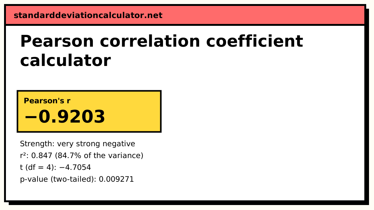
t = r√(n − 2) ÷ √(1 − r²) = −0.920316 × √4 ÷ √(1 − 0.846981) = −4.7054 p = 0.009271 (two-tailed, df = 4)
Probable error of r.
P.E. = 0.6745 × (1 − r²) ÷ √n = 0.6745 × 0.153019 ÷ √6 = 0.042136 6 × P.E. = 0.25281; |r| > 6 P.E.
All three methods give the same r; they differ only in how much arithmetic they save by hand. |t| = 4.705 exceeds 2.776, so the correlation is significant at the 0.05 level: reject H₀.
The formulas
The three standard forms give the same r. Use whichever keeps the arithmetic simplest.
Actual-mean method: r = Σxy ÷ √(Σx² × Σy²), where x = X − X̄ and y = Y − Ȳ
Direct method: r = (NΣXY − ΣXΣY) ÷ √[(NΣX² − (ΣX)²)(NΣY² − (ΣY)²)]
Assumed-mean method: r = (NΣdxdy − ΣdxΣdy) ÷ √[(NΣdx² − (Σdx)²)(NΣdy² − (Σdy)²)], dx = X − A, dy = Y − B
In the first form the lower-case x and y are deviations from the actual means, which is the notation most Indian textbooks use. The assumed-mean form works for any A and B because r does not change when you shift the origin of either variable.
A worked example
The calculator's default data has six pairs: X = 2, 4, 5, 6, 8, 11 and Y = 18, 12, 10, 8, 7, 5.
- Means: X̄ = 36 ÷ 6 = 6 and Ȳ = 60 ÷ 6 = 10. Both are whole numbers, so the actual-mean method is convenient.
- Deviations and their products give Σxy = −67, Σx² = 50 and Σy² = 106.
- r = −67 ÷ √(50 × 106) = −67 ÷ 72.801 = −0.9203.
- Direct method check: ΣX = 36, ΣY = 60, ΣXY = 293, ΣX² = 266, ΣY² = 706, so r = (6 × 293 − 36 × 60) ÷ √[(6 × 266 − 36²)(6 × 706 − 60²)] = −402 ÷ √(300 × 636) = −402 ÷ 436.81 = −0.9203.
- Assumed-mean check with A = 5 and B = 8: Σdx = 6, Σdy = 12, Σdxdy = −55, Σdx² = 56, Σdy² = 130, so r = (6 × (−55) − 6 × 12) ÷ √[(6 × 56 − 36)(6 × 130 − 144)] = −402 ÷ √(300 × 636) = −0.9203.
r² = 0.847, so about 85% of the variation in Y moves in step with X. The t statistic is t = −0.9203 × √4 ÷ √(1 − 0.847) = −4.705 on 4 degrees of freedom, giving p = 0.0093. The critical value at the 5% level is ±2.776, so the correlation is significant. The probable error is 0.6745 × 0.153 ÷ √6 = 0.0421, and |r| is far above 6 × P.E. = 0.253.
Interpreting r
| |r| | Usual description | r² |
|---|---|---|
| 0.9 to 1 | Very strong | 0.81 to 1 |
| 0.7 to 0.9 | Strong | 0.49 to 0.81 |
| 0.5 to 0.7 | Moderate | 0.25 to 0.49 |
| 0.3 to 0.5 | Weak | 0.09 to 0.25 |
| below 0.3 | Negligible | below 0.09 |
These bands are conventions, not rules. What matters as much as the size of r is whether it is significant for your sample size, and whether the scatter plot shows a straight-line pattern at all.
Testing significance
t = r√(n − 2) ÷ √(1 − r²), df = n − 2
The null hypothesis is that the population correlation ρ is zero. Compare |t| with the critical t for n − 2 degrees of freedom, or read the p-value directly. A significant r says the linear association is unlikely to be chance; it does not say the association is strong, and it says nothing about cause.
Common mistakes
- Mixing up Σx² and ΣX². In the actual-mean formula x is a deviation, so Σx² is the sum of squared deviations (50 above), not the sum of squared raw values (266).
- Reading r without the plot. A curved pattern or one outlier can make r misleading. The scatter plot above is there for that reason.
- Treating correlation as causation. Two variables can move together because both depend on a third.
- Rounding the means too early. When the means are long decimals, the assumed-mean method avoids the rounding error that creeps into hand-worked deviations.
For a quicker paste-in version that also reports Spearman's rho and a confidence interval, see the correlation coefficient calculator.
Common questions
What is Karl Pearson's coefficient of correlation?
It is the measure of linear association between two variables, also called the product-moment correlation coefficient and written r. It is the covariance of x and y divided by the product of their standard deviations, so it has no units and always lies between −1 and +1. The sign gives the direction and the size gives the strength of the straight-line relationship.
Do the actual-mean, direct and assumed-mean methods give different answers?
No. They are the same formula rearranged, so they give exactly the same r. The actual-mean method is easiest when the means are whole numbers; the direct method avoids deviations altogether; the assumed-mean (short-cut) method keeps the numbers small when the means are awkward decimals. Any value can serve as the assumed mean. With the default data, A = 5 and B = 8 give r = −0.9203, the same as the other two methods.
What is the probable error of r?
P.E. = 0.6745 × (1 − r²) ÷ √n. It is an older way of judging significance that still appears in Indian commerce and economics syllabi: if |r| is more than six times the probable error, r is taken as significant; if it is less than the P.E., it is not. The t-test reported above is the modern replacement and gives an exact p-value.
How many pairs do I need?
The calculation works from three pairs, but r from a small sample is unstable. With 6 pairs |r| must exceed 0.811 to be significant at the 5% level (two-tailed); with 30 pairs, 0.361 is enough. The confidence interval in the results shows how much the population correlation could differ from your r.
Is r affected by change of origin and scale?
It is unaffected by change of origin (adding or subtracting a constant) and by change of scale (multiplying or dividing by a positive constant). That is why the assumed-mean method works, and why converting heights from centimetres to inches leaves r unchanged. Multiplying one variable by a negative number flips the sign of r but not its size.
Related calculators
-
Correlation coefficient calculator
Pearson's r with Spearman's rho, a confidence interval and a quick paste-in data box.
-
Spearman's rank correlation
Correlation of ranks, for ordinal data or curved relationships.
-
Linear regression calculator
The least-squares line through the same data, with predictions.
-
Kendall's tau
Rank correlation from concordant and discordant pairs.