Quadratic regression calculator
Fit a parabola to paired data. Enter x and y values and the calculator returns the least-squares equation y = ax² + bx + c, how well it fits, and a predicted y for any x you choose.
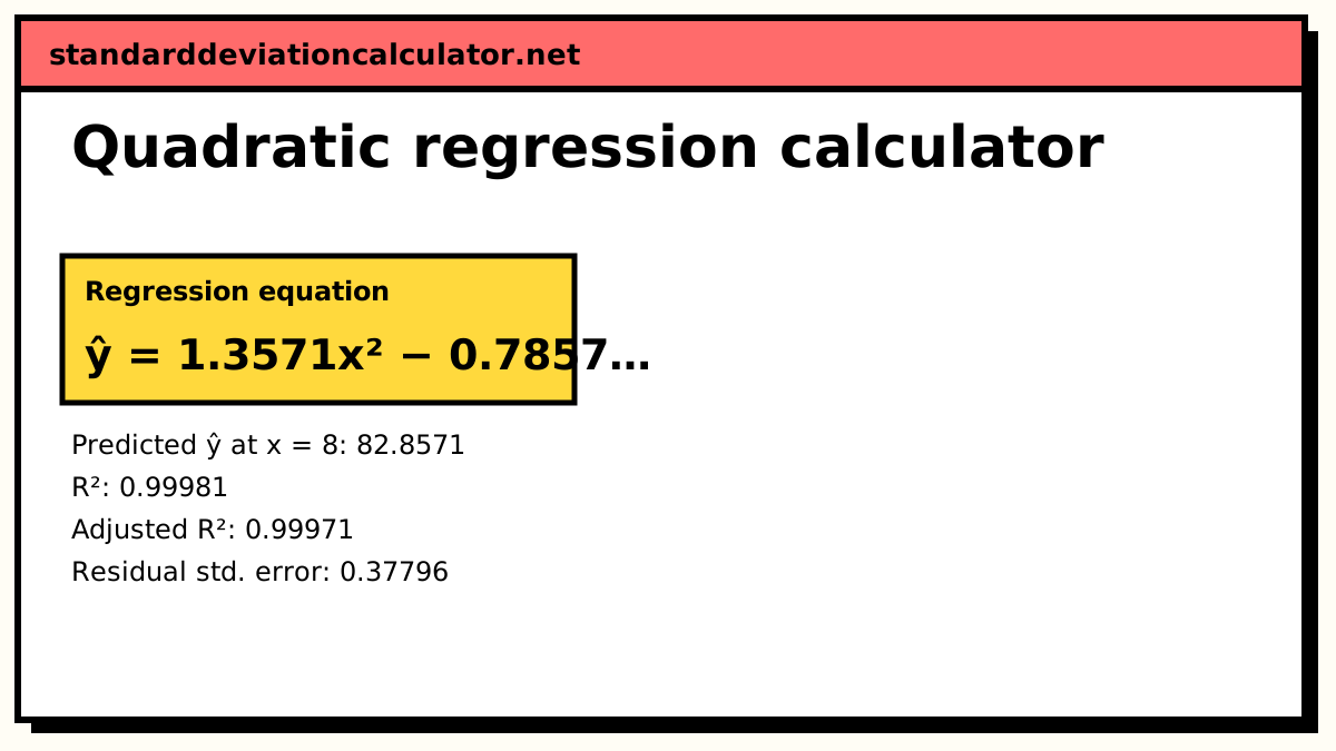
━ Data ━ ŷ = 1.3571x² − 0.78571x + 2.2857
| Term | Coefficient |
|---|---|
| a (x²) | 1.3571429 |
| b (x) | −0.78571429 |
| c (Constant) | 2.2857143 |
| x | y | ŷ | Residual y − ŷ |
|---|---|---|---|
| 1 | 3 | 2.85714 | 0.14286 |
| 2 | 6 | 6.14286 | −0.14286 |
| 3 | 12 | 12.1429 | −0.14286 |
| 4 | 21 | 20.8571 | 0.14286 |
| 5 | 32 | 32.2857 | −0.28571 |
| 6 | 47 | 46.4286 | 0.57143 |
| 7 | 63 | 63.2857 | −0.28571 |
Show the working, step by step
Set up the model ŷ = ax² + bx + c and the design matrix with columns 1, x, x² for the 7 points.
Solve the least-squares problem (minimise Σ(y − ŷ)²). The calculator centres and scales x first and uses a QR decomposition, which gives the same answer as the normal equations with far less rounding error.
ŷ = 1.3571x² − 0.78571x + 2.2857
Split the variation in y.
SST = Σ(y − ȳ)² = 2995.43 SSE = Σ(y − ŷ)² = 0.571429 SSR = SST − SSE = 2994.86
Coefficient of determination and its adjusted form.
R² = 1 − SSE ÷ SST = 1 − 0.571429 ÷ 2995.43 = 0.999809 adjusted R² = 1 − (1 − R²)(n − 1) ÷ (n − 2 − 1) = 1 − 0.000190767 × 6 ÷ 4 = 0.999714
Overall F-test of H₀: every non-constant coefficient is zero.
F = (SSR ÷ 2) ÷ (SSE ÷ 4) = 10482, p < 0.0001
Prediction at x = 8: substitute into the equation.
ŷ(8) = 82.8571
A very close fit: the curve explains 99.98% of the variation in y. Adding degrees always raises R²; compare adjusted R² when choosing the degree.
The model and the normal equations
ŷ = ax² + bx + c, minimise Σ(y − ŷ)²
Setting the derivatives with respect to a, b and c to zero gives three normal equations:
Σy = aΣx² + bΣx + cn Σxy = aΣx³ + bΣx² + cΣx Σx²y = aΣx⁴ + bΣx³ + cΣx²
Solving those by hand is the classroom method. The calculator gets the same a, b and c through a QR decomposition on centred x, which avoids the rounding trouble the power sums cause when x is large.
A worked example
The default data are seven points: x = 1 to 7 and y = 3, 6, 12, 21, 32, 47, 63. The differences between successive y values (3, 6, 9, 11, 15, 16) keep growing, which is the sign of curvature a straight line would miss. The least-squares parabola is
ŷ = 1.3571x² − 0.78571x + 2.2857
As exact fractions these are a = 19/14, b = −11/14 and c = 16/7. The fitted values are 2.86, 6.14, 12.14, 20.86, 32.29, 46.43 and 63.29, so no residual is bigger than 0.43. The squared residuals add to SSE = 0.571 against a total SST = 2995.4, so
R² = 1 − 0.571 ÷ 2995.4 = 0.99981, adjusted R² = 0.99971
The overall F statistic on (2, 4) degrees of freedom is 10,482, with p below 0.0001. The default prediction at x = 8 is ŷ = 1.3571 × 64 − 0.78571 × 8 + 2.2857 = 82.86. Because 8 lies outside the data, the calculator adds a warning. Parabolas bend away quickly beyond the range they were fitted on.
How to interpret the coefficients
The sign of a tells you the shape: positive opens upward (a valley), negative opens downward (a hill). The size of a is how sharply the curve bends. b on its own is the slope of the curve at x = 0, not an average slope over the data, and c is the fitted value at x = 0. If x = 0 is far from your data, neither b nor c has much meaning by itself. To find the slope at any x, use 2ax + b.
Common mistakes
- Reading R² alone. A quadratic always fits at least as well as a line on the same data. Compare adjusted R² and look at the residuals.
- Extrapolating. A parabola predicts that growth keeps accelerating or reverses. Neither may be true outside your data.
- Swapping the columns. Regressing x on y gives a different curve. Put the variable you want to predict in the y column.
- Too few points. Four points leave one degree of freedom, and the R² from so few points tells you very little.
Common questions
What is quadratic regression?
Fitting the parabola y = ax² + bx + c that makes the sum of squared vertical distances from the points to the curve as small as possible. It is still linear regression in the statistical sense, because the model is linear in the unknowns a, b and c; only the predictors x and x² are curved.
How many points do I need?
Three points define a parabola exactly, so a fit needs at least four to leave any degree of freedom for error. With four or five points the R² will be high almost regardless of the data. Ten or more points spread across the range give a far more trustworthy curve.
How do I find the vertex of the fitted parabola?
The turning point is at x = −b ÷ (2a). For the default fit, x = 0.78571 ÷ (2 × 1.3571) = 0.289, which lies just below the smallest x in the data. A vertex far outside the data range is a reminder that the fitted curve is only reliable near the points you gave it.
Should I use a quadratic or a straight line?
Fit both and compare adjusted R² and the residual plots. If the straight-line residuals form a U or an upside-down U, the quadratic is capturing real curvature. If they look random, the extra x² term is not needed.
Does it matter if my x values are large, like years?
Not to this calculator. It centres and scales x before solving and uses a QR decomposition, so x values such as 2015 to 2026 do not lose precision the way the textbook normal equations can. The coefficients it reports are still for the original x.
Related calculators
-
Cubic regression calculator
Fit y = ax³ + bx² + cx + d when the data bends twice.
-
Polynomial regression calculator
Choose any degree from 1 to 6 and compare adjusted R².
-
Linear regression calculator
The straight-line fit, with slope and intercept tests.