Cubic regression calculator
Fit a third-degree polynomial to your data. Enter x and y values to get the least-squares cubic, its R², a chart of the curve through the points and a prediction at any x.
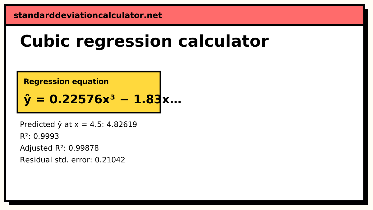
━ Data ━ ŷ = 0.22576x³ − 1.83x² + 4.4607x + 1.2379
| Term | Coefficient |
|---|---|
| a (x³) | 0.22575758 |
| b (x²) | −1.8299784 |
| c (x) | 4.4607143 |
| d (Constant) | 1.2378788 |
| x | y | ŷ | Residual y − ŷ |
|---|---|---|---|
| 0 | 1.2 | 1.23788 | −0.037879 |
| 1 | 4.1 | 4.09437 | 0.0056277 |
| 2 | 4.8 | 4.64545 | 0.15455 |
| 3 | 4.2 | 4.24567 | −0.045671 |
| 4 | 4.1 | 4.24957 | −0.14957 |
| 5 | 5.9 | 6.01169 | −0.11169 |
| 6 | 11.2 | 10.8866 | 0.31342 |
| 7 | 20.1 | 20.2288 | −0.12879 |
Show the working, step by step
Set up the model ŷ = ax³ + bx² + cx + d and the design matrix with columns 1, x, x², x³ for the 8 points.
Solve the least-squares problem (minimise Σ(y − ŷ)²). The calculator centres and scales x first and uses a QR decomposition, which gives the same answer as the normal equations with far less rounding error.
ŷ = 0.22576x³ − 1.83x² + 4.4607x + 1.2379
Split the variation in y.
SST = Σ(y − ȳ)² = 253.58 SSE = Σ(y − ŷ)² = 0.1771 SSR = SST − SSE = 253.403
Coefficient of determination and its adjusted form.
R² = 1 − SSE ÷ SST = 1 − 0.1771 ÷ 253.58 = 0.999302 adjusted R² = 1 − (1 − R²)(n − 1) ÷ (n − 3 − 1) = 1 − 0.000698397 × 7 ÷ 4 = 0.998778
Overall F-test of H₀: every non-constant coefficient is zero.
F = (SSR ÷ 3) ÷ (SSE ÷ 4) = 1907.8, p < 0.0001
Prediction at x = 4.5: substitute into the equation.
ŷ(4.5) = 4.82619
A very close fit: the curve explains 99.93% of the variation in y. Adding degrees always raises R²; compare adjusted R² when choosing the degree.
The model
ŷ = ax³ + bx² + cx + d, minimise Σ(y − ŷ)²
The four coefficients solve four normal equations built from the sums Σx⁰ to Σx⁶ and Σxʲy. Those sums get very large even for modest x, so the calculator solves the same least-squares problem with a QR decomposition on centred and scaled x. The answer is identical and the rounding error is much smaller.
A worked example
The default data are eight readings at x = 0 to 7: y = 1.2, 4.1, 4.8, 4.2, 4.1, 5.9, 11.2, 20.1. The values rise, flatten and dip slightly between x = 2 and x = 4, then climb steeply. That S shape is what a cubic can follow. The least-squares cubic is
ŷ = 0.22576x³ − 1.83x² + 4.4607x + 1.2379
The fitted values are 1.24, 4.09, 4.65, 4.25, 4.25, 6.01, 10.89 and 20.23. The residuals add in squares to SSE = 0.177 against SST = 253.58, so
R² = 1 − 0.177 ÷ 253.58 = 0.9993, adjusted R² = 0.99878
The residual standard error is 0.21, and the F statistic on (3, 4) degrees of freedom is 1,907.8 with p below 0.0001. The default prediction at x = 4.5 is ŷ = 4.83, which sits inside the data range. For comparison, a quadratic on the same data reaches only R² = 0.880 (adjusted 0.832). The cubic term is doing real work here.
How to interpret the result
Read the equation as a whole rather than coefficient by coefficient. The individual terms are strongly correlated with one another (x, x² and x³ all rise together), so each coefficient's size depends on the others. The useful outputs are the fitted curve, the predictions within the data range, the turning points (where 3ax² + 2bx + c = 0) and adjusted R² compared with lower degrees. A cubic that beats a quadratic by a large margin in adjusted R², as here, is picking up a real second bend. A gain in the third decimal place is usually noise.
When a cubic is the wrong choice
Growth that compounds at a steady rate is better described by an exponential curve, and growth that levels off towards a ceiling by a logistic one. A cubic can mimic either over a short stretch but will head the wrong way once it runs past the data. If you have a reason to expect one of those shapes, fit it directly. Use a cubic when you have no theory about the shape and just need a smooth curve through data with two bends.
Common mistakes
- Extrapolating. Outside the data a cubic heads to plus or minus infinity, often in the wrong direction.
- Choosing the degree by R². R² can only rise with degree. Use adjusted R², a residual plot or a hold-out set.
- Rounding coefficients too early. Because x³ is large, rounding a to two decimals can move predictions a lot. Keep the full values the calculator shows.
- Too few points. Five points leave one residual degree of freedom, and the R² from five points means little.
Common questions
When is a cubic the right model?
When the data bend in two directions: rising, levelling off (or dipping), then rising again, or the mirror image. A cubic has up to two turning points and one inflection point. If the data only curve one way, a quadratic is usually enough and easier to explain.
How many data points does a cubic fit need?
At least five. Four points determine a cubic exactly and leave no residual degrees of freedom. With five you get one, which is still very little. Aim for eight or more spread over the range.
Why is the cubic coefficient so small?
Because it multiplies x³, which grows fast. In the default fit a = 0.226, but at x = 7 the term ax³ contributes 0.226 × 343 = 77. The size of a coefficient depends on the units of x, so a small a does not mean the cubic term is unimportant. Compare adjusted R² with and without it.
How do I find the turning points of the fitted cubic?
Differentiate: 3ax² + 2bx + c = 0 and solve that quadratic. For the default fit the derivative is 0.677x² − 3.66x + 4.461, which is zero at about x = 1.9 and x = 3.5: a local peak near x = 1.9 and a trough near x = 3.5, matching the dip in the data.
Related calculators
-
Quadratic regression calculator
The parabola of best fit, for data that curve one way.
-
Polynomial regression calculator
Any degree from 1 to 6, with a table comparing each.
-
Coefficient of determination calculator
R² and adjusted R² from data, predictions or sums of squares.