Coefficient of determination calculator (R-squared)
Find R², the proportion of the variation in y that a model explains. Paste x and y data to fit a straight line, enter actual and predicted values from any model, or type in the sums of squares.
Leave blank to skip adjusted R².
Give SSR or SSE; leave the other blank.
━ Data ━ ŷ = 60.405 + 2.9411x
Show the working, step by step
Fit the least-squares line.
x̄ = 6.875, ȳ = 80.625 slope = Sxy ÷ Sxx = 249.625 ÷ 84.875 = 2.94109 ŷ = 60.405 + 2.9411x
Total variation in y, and the part the line leaves unexplained.
SST = Σ(y − ȳ)² = 755.875 SSE = Σ(y − ŷ)² = 21.7054 SSR = SST − SSE = 734.17
R² is the explained share of the total.
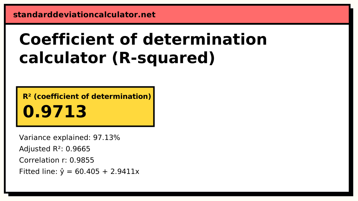
R² = SSR ÷ SST = 734.17 ÷ 755.875 = 0.971284 check: r² = 0.985538² = 0.971284
Adjusted R² with k = 1 predictor.
adjusted R² = 1 − (1 − R²)(n − 1) ÷ (n − k − 1) = 1 − 0.0287157 × 7 ÷ 6 = 0.966498
The line explains 97.13% of the variation in y: a very close fit.
The formula
R² = SSR ÷ SST = 1 − SSE ÷ SST adjusted R² = 1 − (1 − R²)(n − 1) ÷ (n − k − 1)
SST = Σ(y − ȳ)² is the total variation in y. SSE = Σ(y − ŷ)² is what the model leaves unexplained, and SSR = SST − SSE is the part it explains. n is the number of observations and k the number of predictors (k = 1 for a straight line).
A worked example from data
The default table has eight students' hours of revision (x) and exam scores (y): hours 2, 3, 5, 6, 8, 9, 10, 12 and scores 65, 70, 74, 80, 83, 90, 88, 95. The means are x̄ = 6.875 and ȳ = 80.625.
- The least-squares slope is Sxy ÷ Sxx = 249.625 ÷ 84.875 = 2.9411, so the line is ŷ = 60.405 + 2.9411x.
- The total sum of squares is SST = 755.875.
- The residual sum of squares is SSE = 21.705, which leaves SSR = 755.875 − 21.705 = 734.17.
- R² = 734.17 ÷ 755.875 = 0.9713.
- Adjusted R² = 1 − 0.0287 × 7 ÷ 6 = 0.9665.
Hours of revision explain about 97% of the variation in these scores. As a check, Pearson's r is 0.9855, and 0.9855² = 0.9713.
From actual and predicted values
If a model has already made predictions, choose the second mode. The default rows compare six actual values (12, 15, 19, 22, 25, 31) with a model's predictions (11.5, 15.8, 18.2, 23.1, 24.4, 29.8). The squared errors add to SSE = 4.54, the actual values vary by SST = 237.33 around their mean of 20.67, and R² = 1 − 4.54 ÷ 237.33 = 0.9809. This mode is the one to use on a hold-out test set, where R² can fall below zero.
From sums of squares
Regression output often prints the ANOVA table rather than R². With SSR = 320 and SST = 400, R² = 320 ÷ 400 = 0.80. With n = 25 and one predictor, adjusted R² = 1 − 0.2 × 24 ÷ 23 = 0.7913. If you have SSE instead, leave SSR blank: R² = 1 − SSE ÷ SST.
How to read R²
R² runs from 0 (the model does no better than the mean) to 1 (every point lies on the fitted values). The calculator labels values above 0.9 as a very close fit and below 0.1 as almost no fit, but those labels are only a rough guide. A high R² does not prove the model is right: a straight line fitted to curved data can still have a high R² while the residuals show an obvious pattern. A low R² does not mean a slope is zero either. With enough data a real but small effect can be highly significant and still explain only a little of the variation.
Common mistakes
- Comparing plain R² across models of different size. Adding predictors always raises R². Use adjusted R² or a test set.
- Treating R² as the slope's significance. Significance comes from the t- or F-test, which also depends on n.
- Squaring r for a model with several predictors. r² equals R² only for one predictor. With several, compute 1 − SSE/SST.
- Mixing up SSR and SSE. Some books write SSR for the residual sum of squares. Check which one your source means before dividing.
Common questions
What does R² actually measure?
The share of the variation in y, measured as the sum of squared deviations from the mean, that the model accounts for. R² = 0.97 means the fitted values explain 97% of that variation and the residuals hold the other 3%. It says nothing about whether the model is causal or whether a straight line was the right shape to fit.
Is R² the same as r squared?
For a straight line fitted by least squares with an intercept, yes: R² equals the square of Pearson's r between x and y. In the default example r = 0.9855 and r² = 0.9713. For multiple regression R² is the square of the correlation between y and the fitted values, and for predictions that did not come from a least-squares fit to the same rows the two numbers differ.
Can R² be negative?
Not for a least-squares fit with an intercept on the data it was fitted to. It can be negative when you compute 1 − SSE/SST for predictions from somewhere else (a test set, a model without an intercept, a forecast). A negative value means the predictions do worse than simply guessing the mean of y every time.
When should I report adjusted R² instead?
When you compare models with different numbers of predictors. Plain R² never goes down when you add a predictor, even a useless one. Adjusted R² = 1 − (1 − R²)(n − 1)/(n − k − 1) charges for each extra predictor and falls if the new one adds less than it costs.
What is a good R² value?
It depends on the field. Physical measurements often give R² above 0.95; models of human behaviour can be useful at 0.2. Judge a model by its residual plot, its prediction error in the units of y, and whether the predictors make sense, not by a single R² cut-off.
Related calculators
-
Linear regression calculator
Slope, intercept, standard errors and the t-test for a straight-line fit.
-
Multiple regression calculator
R² and adjusted R² with up to four predictors.
-
Correlation coefficient calculator
Pearson's r, whose square is R² for a simple linear fit.