Residual calculator
Enter (x, y) data to see how far each point sits from the regression line. The calculator fits the least-squares line, or uses a slope and intercept you give it, and lists every residual with a plot.
| x | y | ŷ | e = y − ŷ | e² |
|---|---|---|---|---|
| 1 | 2.1 | 2 | 0.1 | 0.01 |
| 2 | 3.9 | 4.02 | −0.12 | 0.0144 |
| 3 | 6.2 | 6.04 | 0.16 | 0.0256 |
| 4 | 7.8 | 8.06 | −0.26 | 0.0676 |
| 5 | 10.1 | 10.08 | 0.02 | 0.0004 |
| 6 | 12.2 | 12.1 | 0.1 | 0.01 |
| Sum | 0 | 0.128 |
┄ e = 0
Show the working, step by step
Fit the least-squares line: b = Sxy/Sxx and a = ȳ − b·x̄.
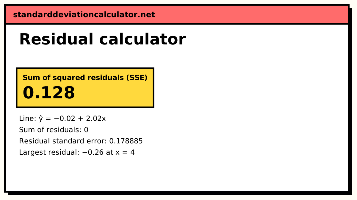
ŷ = −0.02 + 2.02x
Predict y at each x. For the first point, x = 1:
ŷ = −0.02 + 2.02 × 1 = 2
Subtract the prediction from the observed value.
e = y − ŷ = 2.1 − 2 = 0.1
Square the residuals and add them.
SSE = 0.1² + (−0.12)² + 0.16² + (−0.26)² + 0.02² + 0.1² = 0.128
For a least-squares line with an intercept, the residuals always sum to zero. Look at the plot instead: a curve or a funnel shape means the straight line is not a good model.
The formula
ŷ = a + b·x e = y − ŷ SSE = Σe²
For the least-squares line, b = Sxy ÷ Sxx and a = ȳ − b·x̄, where Sxy = Σ(x − x̄)(y − ȳ) and Sxx = Σ(x − x̄)². Least squares chooses a and b to make SSE as small as possible.
A worked example
The default data are six points: (1, 2.1), (2, 3.9), (3, 6.2), (4, 7.8), (5, 10.1) and (6, 12.2). Here x̄ = 3.5 and ȳ = 7.05, Sxx = 17.5 and Sxy = 35.35, so b = 35.35 ÷ 17.5 = 2.02 and a = 7.05 − 2.02 × 3.5 = −0.02. The fitted line is ŷ = −0.02 + 2.02x.
| x | y | ŷ | e = y − ŷ |
|---|---|---|---|
| 1 | 2.1 | 2.00 | 0.10 |
| 2 | 3.9 | 4.02 | −0.12 |
| 3 | 6.2 | 6.04 | 0.16 |
| 4 | 7.8 | 8.06 | −0.26 |
| 5 | 10.1 | 10.08 | 0.02 |
| 6 | 12.2 | 12.10 | 0.10 |
The residuals sum to zero, as they must for a least-squares fit. Squaring and adding them gives SSE = 0.01 + 0.0144 + 0.0256 + 0.0676 + 0.0004 + 0.01 = 0.128, and the residual standard error is √(0.128 ÷ 4) = 0.179. The biggest miss is at x = 4, where the point sits 0.26 below the line.
Reading the residual plot
The plot puts x on the horizontal axis and the residual on the vertical axis, with a line at zero. For the default data the points bounce above and below zero with no pattern, and they are all small compared with the y values, so a straight line describes these data well.
Patterns are what to look for. Residuals that are positive at both ends and negative in the middle trace a U shape and mean the data curve; a quadratic or a transformation will fit better. Residuals whose spread grows with x mean the variability is not constant, which makes the usual standard errors and p-values unreliable. A point with a residual several times larger than the rest deserves a second look before it is kept.
To check someone else's line, switch to "I have the slope and intercept". The residuals of a line that is not the least-squares fit will not sum to zero, and its SSE will be larger than 0.128.
Residuals and R²
SSE is the part of the variation in y that the line leaves unexplained. Dividing it by the total sum of squares, Σ(y − ȳ)², and subtracting from 1 gives R². Here Σ(y − ȳ)² = 71.535, so R² = 1 − 0.128 ÷ 71.535 = 0.998.
Common mistakes
- Subtracting the wrong way round. The residual is observed minus predicted, y − ŷ.
- Measuring the distance at right angles to the line. Residuals are vertical distances.
- Judging fit from the sum of residuals. It is always 0 for least squares; use SSE or the plot.
- Rounding the slope and intercept heavily before computing residuals, which leaves them not quite summing to zero.
Common questions
What is a residual?
The vertical distance between an observed point and the regression line: e = y − ŷ, the actual y minus the y the line predicts at that x. A positive residual means the point lies above the line; a negative one means it lies below.
Why do the residuals add up to zero?
For a least-squares line with an intercept, the line always passes through (x̄, ȳ), and the fitting equations force Σe = 0 and Σxe = 0. If you enter your own slope and intercept, the residuals will only sum to zero if that line happens to be the least-squares one.
What should a good residual plot look like?
A shapeless horizontal band around zero, with roughly equal spread at every x. A curve suggests the relationship is not linear; a funnel that widens or narrows suggests the variance changes with x; a single far-off point is a possible outlier.
What is the residual standard error?
√(SSE ÷ (n − 2)), the typical size of a residual. It divides by n − 2 because a straight line uses up two degrees of freedom (the slope and the intercept).
Related calculators
-
Linear regression calculator
Slope, intercept, r and R² for a least-squares line.
-
MSE calculator
MSE, RMSE, MAE and MAPE for any set of predictions.
-
Sum of squares calculator
Total, regression and residual sums of squares.