P-hat calculator (sample proportion)
Enter the number of successes and the sample size to get the sample proportion p̂, its standard error, and a confidence interval for the population proportion.
How many in the sample have the trait.
Show the working, step by step
Divide the successes by the sample size.
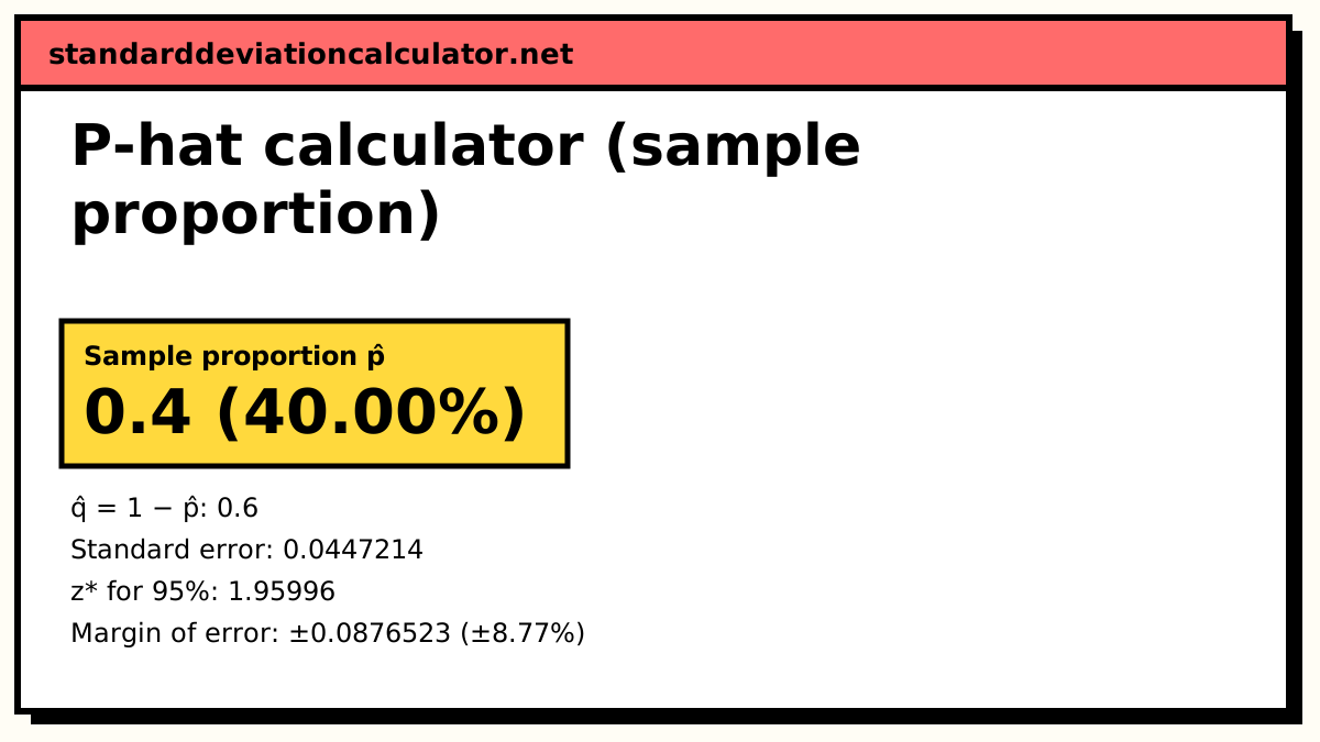
p̂ = x ÷ n = 48 ÷ 120 = 0.4
Standard error of p̂:
SE = √(p̂(1 − p̂) ÷ n) = √(0.4 × 0.6 ÷ 120) = 0.0447214
Margin of error at 95% confidence:
E = z* × SE = 1.95996 × 0.0447214 = 0.0876523
Confidence interval:
p̂ ± E = 0.4 ± 0.0876523 = (0.312348, 0.487652)
Check the conditions for the normal approximation.
n·p̂ = 48 ≥ 10, n·(1 − p̂) = 72 ≥ 10
The Wilson interval adds z²/2n to the successes before centring, which keeps it inside 0 to 1 and gives better coverage when p̂ is near 0 or 1.
The formulas
p̂ = x ÷ n SE = √(p̂(1 − p̂) ÷ n) CI = p̂ ± z* × SE
Here x is the number of successes (people who said yes, parts that passed, patients who recovered), n is the sample size and z* is the critical value for the confidence level: 1.645 for 90%, 1.960 for 95% and 2.576 for 99%.
A worked example
In a survey of 120 customers, 48 say they would buy a new product. The sample proportion is
p̂ = 48 ÷ 120 = 0.4
so 40% of the sample said yes. The standard error is
SE = √(0.4 × 0.6 ÷ 120) = √0.002 = 0.0447214
At 95% confidence the margin of error and interval are
E = 1.95996 × 0.0447214 = 0.0876523 0.4 ± 0.0877 → 0.312 to 0.488
The conditions hold: 48 successes and 72 failures are both at least 10. The Wilson interval, 0.317 to 0.489, is almost the same and slightly shifted toward 0.5, as expected.
How to interpret the result
We are 95% confident that between about 31% and 49% of all customers would buy the product. “95% confident” describes the method: if you repeated the survey many times, about 95% of the intervals built this way would contain the true proportion. It does not mean there is a 95% chance the true value lies in this particular interval.
The interval is wide (almost ±9 points) because 120 responses is a small sample. The margin shrinks with √n, so to halve it to about ±4.4 points you would need four times as many responses, around 480. The standard error is largest when p̂ = 0.5, which is why sample size planning often assumes 0.5 when nothing better is known.
Changing the confidence level
A higher confidence level gives a wider interval from the same data. With 48 of 120, the 90% interval uses z* = 1.645 and runs from about 0.326 to 0.474; the 99% interval uses z* = 2.576 and runs from about 0.285 to 0.515. None of these changes p̂ itself, which stays at 0.4. Pick the level before looking at the data, and report it with the interval.
The same p̂ and standard error feed a one-proportion z-test. To test whether the true share is 50%, compute z = (0.4 − 0.5) ÷ √(0.5 × 0.5 ÷ 120) = −2.19, using the hypothesised 0.5 in the standard error rather than p̂.
Common mistakes
- Using percentages in the formula. Work with 0.4, not 40, or the standard error comes out ten times too large.
- Ignoring the success–failure condition. With 3 successes in 20 the simple interval is unreliable; use the Wilson interval.
- Using the t distribution. Intervals for a proportion use z*, not t*.
- Forgetting that the survey must be random. The interval measures sampling error only, not bias from who chose to respond.
Common questions
What is p-hat?
p̂ (“p-hat”) is the sample proportion: the number of successes x divided by the sample size n. It estimates the population proportion p, which is usually unknown. If 48 of 120 people surveyed say yes, p̂ = 48 ÷ 120 = 0.4.
What is the standard error of p-hat?
SE = √(p̂(1 − p̂) ÷ n). It measures how much p̂ would vary from sample to sample. For p̂ = 0.4 and n = 120 it is √(0.24 ÷ 120) = 0.0447. Quadrupling the sample size halves it.
When can I use the normal approximation?
When there are at least 10 successes and 10 failures in the sample (some textbooks use 5). Below that, the sampling distribution of p̂ is too skewed and the simple interval can have poor coverage or run past 0 or 1. The calculator warns you and also gives the Wilson interval.
What is the Wilson interval?
A confidence interval for a proportion that stays inside 0 to 1 and has closer to the stated coverage for small samples or proportions near 0 or 1. It pulls the centre slightly toward 0.5. For large samples it agrees closely with the usual p̂ ± z·SE interval.
What is the difference between p-hat and a p-value?
They are unrelated despite the similar names. p̂ is an estimate of a proportion. A p-value is the probability, under a null hypothesis, of a result at least as extreme as the one observed.
Related calculators
-
Margin of error
The ± part of a survey result, for means or proportions.
-
Confidence interval
Intervals for a mean from data or summary statistics.
-
Sample size calculator
How many responses you need for a target margin.