Chebyshev's theorem calculator
Find the smallest share of any data set that must lie within k standard deviations of its mean. Enter k, a target percentage or an interval, and compare the answer with a normal distribution.
Must be more than 1 for a useful bound.
━ Chebyshev minimum, any distribution ┄ Normal distribution (empirical rule)
| k | Chebyshev (any shape) | Normal (empirical rule) |
|---|---|---|
| 1.5 | 55.56% | 86.64% |
| 2 | 75.00% | 95.45% |
| 2.5 | 84.00% | 98.76% |
| 3 | 88.89% | 99.73% |
| 4 | 93.75% | 99.99% |
Show the working, step by step
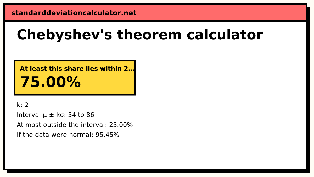
k = 2 standard deviations.
Chebyshev’s theorem: for any distribution with a finite variance, at least 1 − 1/k² of the values lie within k standard deviations of the mean.
1 − 1/k² = 1 − 1/2² = 1 − 0.25 = 75.00%
The interval itself:
μ − kσ = 70 − 2 × 8 = 54 μ + kσ = 70 + 2 × 8 = 86
For comparison, a normal distribution puts much more inside the same interval:
P(|Z| < 2) = 95.45%
Chebyshev gives a floor that holds for every shape of distribution, so it is cautious. Use the empirical rule only when you know the data are roughly bell-shaped.
The formula
P(|X − μ| < kσ) ≥ 1 − 1/k², k > 1
Equivalently, at most 1/k² of the values lie k or more standard deviations from the mean. Rearranged for k, a target share p needs k = 1 ÷ √(1 − p).
A worked example
Exam scores have a mean of 70 and a standard deviation of 8, and you know nothing about the shape of the distribution. What share of students scored between 54 and 86?
Both ends are 16 points, or 2 standard deviations, from the mean, so k = 2:
1 − 1/2² = 1 − 0.25 = 0.75
At least 75% of the students scored between 54 and 86, whatever the distribution looks like. At most 25% scored outside that range. If the scores happened to be normal, the share would be about 95.45%, which is the empirical rule's figure. The chart plots both curves so you can see the gap at every k.
The “interval” mode does the same in reverse. The second default asks about 58 to 82: that is 12 points, or 1.5 SDs, either side of 70, so at least 1 − 1/1.5² = 55.56% of scores lie in it. The “percentage” mode answers questions such as “how wide must the interval be to catch 90%?”: k = 1 ÷ √0.1 = 3.162, so 70 ± 3.162 × 8, from 44.70 to 95.30.
How to interpret the result
The answer is a floor, not an estimate. Real data sets nearly always have more inside the interval than Chebyshev guarantees. Use the theorem when you cannot assume a shape: skewed incomes, waiting times, or any data you have only as a mean and standard deviation. When the data are roughly bell-shaped, the empirical rule gives a much tighter and more useful answer.
| k | Chebyshev minimum | Normal distribution |
|---|---|---|
| 1.5 | 55.56% | 86.64% |
| 2 | 75.00% | 95.45% |
| 3 | 88.89% | 99.73% |
| 4 | 93.75% | 99.99% |
The bound is sharp: for any k there is a distribution that puts exactly 1/k² of its values at μ ± kσ and the rest at μ, and then the share strictly inside the interval is exactly 1 − 1/k².
Where the bound comes from
The variance is the average squared distance from the mean. Every value k or more standard deviations away contributes at least k²σ² to that average. If a share q of the values were that far out, the variance would be at least q × k²σ², and it cannot be more than σ², so q ≤ 1/k². That one line is the whole proof, and it explains why the theorem needs nothing about the shape of the distribution.
Common mistakes
- Reading 75% as “75% of the data”. It is at least 75%; the true share could be anywhere up to 100%.
- Using k ≤ 1. The theorem then says nothing; the calculator reports a bound of 0%.
- Applying it to a lopsided interval. Measure k from the nearer end, or the bound can be wrong.
- Using the empirical rule on skewed data. If you do not know the shape, Chebyshev is the safe choice.
Common questions
What does Chebyshev's theorem say?
For any distribution with a finite mean and standard deviation, at least 1 − 1/k² of the values lie within k standard deviations of the mean, for every k greater than 1. At k = 2 that is at least 75%, and at k = 3 at least 88.9%.
How is Chebyshev's theorem different from the empirical rule?
The empirical rule (68–95–99.7) applies only to bell-shaped, roughly normal data and gives approximate shares. Chebyshev's theorem applies to every distribution, however skewed, and gives a guaranteed minimum. The price of that generality is that its bounds are much lower: 75% within 2 SDs instead of about 95%.
Why does the theorem need k greater than 1?
At k = 1 the formula gives 1 − 1 = 0, and below 1 it goes negative. Both are true but useless: there are distributions with no values at all strictly within one standard deviation of the mean (half at μ − σ and half at μ + σ, for example).
How do I find k for a given percentage?
Solve 1 − 1/k² = p, which gives k = 1 ÷ √(1 − p). To guarantee at least 90% of the data, k = 1 ÷ √0.1 = 3.162 standard deviations. Choose “The percentage I want to cover” in the calculator.
Can I use Chebyshev for an interval that is not centred on the mean?
Only by shrinking it to a centred one. The theorem covers intervals μ ± kσ, so the calculator takes k from the side closer to the mean. The true share inside the wider, lopsided interval is at least that much, and possibly more.
Related calculators
-
Empirical rule calculator
The 68–95–99.7 rule for bell-shaped data.
-
Z-score calculator
How many standard deviations a value is from the mean.
-
Normal distribution
Exact areas under the bell curve.