How to interpret standard deviation
A standard deviation on its own answers nothing. "SD = 12.4" becomes useful only once you know its units, what it is being compared with, how many values produced it and whether a couple of extreme points are behind it. This page is a checklist for turning the number into a sentence you can defend.
If you need the definition first, start with what standard deviation is. The steps below assume you already have a result and want to know what it says. They use one running example: the delivery times, in minutes, of 20 orders from a single restaurant last month. The data is loaded in the calculator so you can check every figure.
Separate numbers with commas, spaces or new lines, or paste a spreadsheet column.
Decimals and negatives are fine; write 10:3 for a value that occurs 3 times.
Your results will appear here: the standard deviation first, then the rest of the summary and a chart.
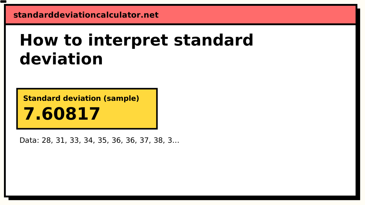
Standard deviation (sample)
7.60817
7.61
Your values typically sit about 7.61 above or below their mean of 40.1, in the same units as your data. 15 of 20 values (75%) fall between 32.49 and 47.71, within one standard deviation of the mean; for normally distributed data about 68% would.
Population SD (σ): 7.41552, if these values are the whole group.
- Count (n)
- 20
- Mean (x̄)
- 40.1
- Variance (s²)
- 57.8842
- Standard error
- 1.70124
- Minimum
- 28
- Q1 (25%)
- 35.75
- Median
- 38.5
- Q3 (75%)
- 43.25
- Maximum
- 61
- Range
- 33
More statistics (5)
- Relative SD (%RSD)
- 18.973%
- Coefficient of variation
- 0.18973
- Sum (Σx)
- 802
- Sum of squares, Σ(x − x̄)²
- 1099.8
- IQR (Q3 − Q1)
- 7.5
Data distribution
Shaded bands mark ±1, ±2 and ±3 SD from the mean. 15 of 20 values (75%) fall within ±1 SD.
Chart as text
Mean 40.1, sample standard deviation s = 7.60817, from 20 values between 28 and 61.
- Within ±1 SD (32.49 to 47.71): 15 of 20 values (75%). About 68% for normal data.
- Within ±2 SD: 19 (95%). About 95% for normal data.
- Within ±3 SD: 20 (100%). About 99.7% for normal data.
Show the working, step by step
Step 1: pin down units, scale and version
The standard deviation is in the same units as the data, so write the unit down before anything else. For the deliveries the mean is 802 ÷ 20 = 40.1 minutes and the sample standard deviation is 7.61 minutes. Also confirm which version you have. The sample SD (divide by n − 1) is 7.61; the population SD (divide by n) is 7.42. For 20 orders standing in for the restaurant's usual performance, the sample version is the right one; the sample vs population page explains the choice.
Scale also means the possible range of the measurement. An SD of 12.4 on a test marked out of 100 is a wide spread; the same 12.4 on a 1,000-point scale is narrow.
Step 2: compare it with the mean
Dividing the SD by the mean gives the coefficient of variation, which removes the unit:
CV = s / x̄ = 7.61 / 40.1 = 0.190 = 19.0%
A typical delivery differs from the average by about a fifth of the average. That is easier to reason about than "7.61 minutes", and it lets you compare spread across things measured differently. Two caveats. There is no universal "good" CV: an analytical lab may reject a method above 2%, while 20% is ordinary for delivery times, sales or reaction times. And the CV only makes sense for data with a true zero; a CV of temperatures in °C changes if you switch to °F, so it means nothing.
Step 3: sanity-check it against the range
A quick way to catch a wrong input or a wrong formula is the range rule of thumb. For moderately sized, roughly bell-shaped data, the standard deviation is usually somewhere near a quarter of the range. For large samples (hundreds of values) the range stretches further and a sixth of the range is the closer guide.
range = 61 − 28 = 33 range / 4 = 8.25 range / 6 = 5.5
The computed 7.61 sits comfortably near 8.25, so nothing looks off. This is a rough check, not an estimate to report. If your SD is several times larger or smaller than range ÷ 4, look for a typo, a unit mix-up or a variance reported as an SD. The range calculator gives the minimum, maximum and range in one step.
Step 4: compare with a benchmark, a specification or last period
The most useful comparison is with something you already care about. The restaurant promises delivery within 50 minutes. With a mean of 40.1 and an SD of 7.61, the limit is (50 − 40.1) ÷ 7.61 = 1.30 standard deviations above the mean. If the times were normally distributed, about 9.7% of orders would run late; in the data, 2 of 20 (10%) did. The SD has turned into a late-delivery rate, which is what the owner actually wants to know.
The other common comparison is with a previous period. Suppose the month before had an SD of 5.9 minutes. Has the service become less consistent? Step 7 shows why 20 orders are not enough to say so with confidence.
Step 5: use z-scores to place individual values
The standard deviation is also a ruler for single observations. A z-score divides a value's distance from the mean by the SD:
z(61) = (61 − 40.1) / 7.61 = 2.75 z(28) = (28 − 40.1) / 7.61 = −1.59
The 28-minute order was quick but unremarkable. The 61-minute order is almost three standard deviations out, and worth a look at what happened. For bell-shaped data, the 68–95–99.7 rule says how often values that far out should appear; that page covers it, so it is not repeated here.
Step 6: separate what it says about individuals from what it says about the average
The 7.61 minutes describes how much individual deliveries vary. It does not describe how precisely you know the average. That is the standard error:
SE = s / √n = 7.61 / √20 = 1.70 minutes
With the t critical value for 19 degrees of freedom (2.093), the 95% confidence interval for the mean delivery time is 40.1 ± 3.56, or 36.5 to 43.7 minutes. So the typical order is somewhere around 40 minutes, but any one order could easily land 8 minutes either side of that. Mixing the two up is the most common interpretation error in published work: the standard error shrinks as you collect more data, the standard deviation does not.
Step 7: ask how stable the SD itself is
A standard deviation from a small sample is itself uncertain, more than most people assume. The confidence interval for the true σ comes from the chi-square distribution, and its width depends only on n:
| n | 95% CI for σ, as a multiple of s |
|---|---|
| 5 | 0.60 to 2.87 |
| 10 | 0.69 to 1.83 |
| 20 | 0.76 to 1.46 |
| 50 | 0.84 to 1.25 |
| 100 | 0.88 to 1.16 |
| 1,000 | 0.96 to 1.05 |
For the deliveries, 7.61 × 0.76 and 7.61 × 1.46 give a 95% interval for σ of about 5.8 to 11.1 minutes. Last month's 5.9 sits inside it, so this data alone does not show that consistency has got worse. The interval assumes roughly normal data, and skew makes it less trustworthy; the confidence interval for standard deviation calculator does the exact calculation for your own n.
Step 8: check for skew and outliers
Squaring the deviations gives far-out values a lot of weight. Compare the SD with measures that ignore the extremes:
| Statistic | Value (minutes) |
|---|---|
| Mean | 40.1 |
| Median | 38.5 |
| Standard deviation | 7.61 |
| Interquartile range (Q1 35.75, Q3 43.25) | 7.5 |
| IQR ÷ 1.349 (the SD a normal curve with this IQR would have) | 5.56 |
| SD with the 61-minute order removed | 5.96 |
The mean sits above the median and the SD is well above what the middle half of the data implies: the data has a long right tail, as delivery times usually do. The 61 is above the upper IQR fence of 43.25 + 1.5 × 7.5 = 54.5, and removing that one order drops the SD from 7.61 to 5.96. Do not delete it to get a nicer number. Report that one late order accounts for a large share of the spread, and give the median and IQR alongside the mean and SD. (Quartile methods differ between tools; the values here use the inclusive method, and others give an IQR of 8.5.)
Step 9: write the interpretation
A good write-up states the numbers with units and n, gives them a meaning in plain terms, makes the comparison and flags anything that distorts the figure. For the deliveries:
Delivery times last month averaged 40.1 minutes (SD 7.6, n = 20; median 38.5, IQR 7.5). Most orders arrived within about 8 minutes of the average, and 2 of 20 missed the 50-minute promise. One 61-minute order accounts for much of the spread; without it the SD is 6.0. The SD is higher than last month's 5.9, but with 20 orders the difference is within sampling noise (95% CI for σ: 5.8–11.1).
Avoid "the data has a high standard deviation" with no reference point, avoid reporting the standard error as if it were the SD, and avoid more decimal places than the data supports. For the difference between a high and a low SD on the same mean, the two-dataset comparison shows it side by side.
Related calculators
-
What is standard deviation?
The definition, the units, and what high, low and zero mean.
-
Coefficient of variation calculator
The SD as a percentage of the mean, for comparing spread across scales.
-
Confidence interval for SD
How far the true standard deviation could be from the one you measured.
-
Z-score calculator
Place any single value as a number of standard deviations from the mean.
Frequently asked questions about how to interpret standard deviation
Common questions
Can standard deviation be zero?
Standard deviation tells you how much individual values typically differ from the mean. Values within one SD are 'typical'; beyond two or three are unusual. In a normal distribution, 68% of values fall within ±1 SD, 95% within ±2 SD, and 99.7% within ±3 SD. See how to interpret standard deviation for a complete guide.
Can standard deviation be negative?
Standard deviation tells you how much individual values typically differ from the mean. Values within one SD are 'typical'; beyond two or three are unusual. In a normal distribution, 68% of values fall within ±1 SD, 95% within ±2 SD, and 99.7% within ±3 SD. See how to interpret standard deviation for a complete guide.
How should I interpret a low standard deviation in education?
Standard deviation tells you how much individual values typically differ from the mean. Values within one SD are 'typical'; beyond two or three are unusual. In a normal distribution, 68% of values fall within ±1 SD, 95% within ±2 SD, and 99.7% within ±3 SD. See how to interpret standard deviation for a complete guide.
How should I interpret a low standard deviation in exam scores?
Standard deviation tells you how much individual values typically differ from the mean. Values within one SD are 'typical'; beyond two or three are unusual. In a normal distribution, 68% of values fall within ±1 SD, 95% within ±2 SD, and 99.7% within ±3 SD. See how to interpret standard deviation for a complete guide.
How should I interpret a low standard deviation in biology?
Standard deviation tells you how much individual values typically differ from the mean. Values within one SD are 'typical'; beyond two or three are unusual. In a normal distribution, 68% of values fall within ±1 SD, 95% within ±2 SD, and 99.7% within ±3 SD. See how to interpret standard deviation for a complete guide.
How should I interpret a low standard deviation in chemistry?
Standard deviation tells you how much individual values typically differ from the mean. Values within one SD are 'typical'; beyond two or three are unusual. In a normal distribution, 68% of values fall within ±1 SD, 95% within ±2 SD, and 99.7% within ±3 SD. See how to interpret standard deviation for a complete guide.
How should I interpret a low standard deviation in physics?
Standard deviation tells you how much individual values typically differ from the mean. Values within one SD are 'typical'; beyond two or three are unusual. In a normal distribution, 68% of values fall within ±1 SD, 95% within ±2 SD, and 99.7% within ±3 SD. See how to interpret standard deviation for a complete guide.
How should I interpret a low standard deviation in economics?
Standard deviation tells you how much individual values typically differ from the mean. Values within one SD are 'typical'; beyond two or three are unusual. In a normal distribution, 68% of values fall within ±1 SD, 95% within ±2 SD, and 99.7% within ±3 SD. See how to interpret standard deviation for a complete guide.
How should I interpret a low standard deviation in business analytics?
Standard deviation tells you how much individual values typically differ from the mean. Values within one SD are 'typical'; beyond two or three are unusual. In a normal distribution, 68% of values fall within ±1 SD, 95% within ±2 SD, and 99.7% within ±3 SD. See how to interpret standard deviation for a complete guide.
How should I interpret a low standard deviation in manufacturing?
Standard deviation tells you how much individual values typically differ from the mean. Values within one SD are 'typical'; beyond two or three are unusual. In a normal distribution, 68% of values fall within ±1 SD, 95% within ±2 SD, and 99.7% within ±3 SD. See how to interpret standard deviation for a complete guide.
How should I interpret a low standard deviation in quality control?
Standard deviation tells you how much individual values typically differ from the mean. Values within one SD are 'typical'; beyond two or three are unusual. In a normal distribution, 68% of values fall within ±1 SD, 95% within ±2 SD, and 99.7% within ±3 SD. See how to interpret standard deviation for a complete guide.
How should I interpret a low standard deviation in health research?
Standard deviation tells you how much individual values typically differ from the mean. Values within one SD are 'typical'; beyond two or three are unusual. In a normal distribution, 68% of values fall within ±1 SD, 95% within ±2 SD, and 99.7% within ±3 SD. See how to interpret standard deviation for a complete guide.
How should I interpret a low standard deviation in sports performance?
Standard deviation tells you how much individual values typically differ from the mean. Values within one SD are 'typical'; beyond two or three are unusual. In a normal distribution, 68% of values fall within ±1 SD, 95% within ±2 SD, and 99.7% within ±3 SD. See how to interpret standard deviation for a complete guide.
How should I interpret a low standard deviation in weather data?
Standard deviation tells you how much individual values typically differ from the mean. Values within one SD are 'typical'; beyond two or three are unusual. In a normal distribution, 68% of values fall within ±1 SD, 95% within ±2 SD, and 99.7% within ±3 SD. See how to interpret standard deviation for a complete guide.
How should I interpret a low standard deviation in agriculture?
Standard deviation tells you how much individual values typically differ from the mean. Values within one SD are 'typical'; beyond two or three are unusual. In a normal distribution, 68% of values fall within ±1 SD, 95% within ±2 SD, and 99.7% within ±3 SD. See how to interpret standard deviation for a complete guide.
How should I interpret a low standard deviation in machine learning?
Standard deviation tells you how much individual values typically differ from the mean. Values within one SD are 'typical'; beyond two or three are unusual. In a normal distribution, 68% of values fall within ±1 SD, 95% within ±2 SD, and 99.7% within ±3 SD. See how to interpret standard deviation for a complete guide.
How should I interpret a low standard deviation in data science?
Standard deviation tells you how much individual values typically differ from the mean. Values within one SD are 'typical'; beyond two or three are unusual. In a normal distribution, 68% of values fall within ±1 SD, 95% within ±2 SD, and 99.7% within ±3 SD. See how to interpret standard deviation for a complete guide.
How should I interpret a low standard deviation in clinical trials?
Standard deviation tells you how much individual values typically differ from the mean. Values within one SD are 'typical'; beyond two or three are unusual. In a normal distribution, 68% of values fall within ±1 SD, 95% within ±2 SD, and 99.7% within ±3 SD. See how to interpret standard deviation for a complete guide.
How should I interpret a low standard deviation in survey results?
Standard deviation tells you how much individual values typically differ from the mean. Values within one SD are 'typical'; beyond two or three are unusual. In a normal distribution, 68% of values fall within ±1 SD, 95% within ±2 SD, and 99.7% within ±3 SD. See how to interpret standard deviation for a complete guide.
How should I interpret a low standard deviation in customer satisfaction?
Standard deviation tells you how much individual values typically differ from the mean. Values within one SD are 'typical'; beyond two or three are unusual. In a normal distribution, 68% of values fall within ±1 SD, 95% within ±2 SD, and 99.7% within ±3 SD. See how to interpret standard deviation for a complete guide.
How should I interpret a low standard deviation in daily temperatures?
Standard deviation tells you how much individual values typically differ from the mean. Values within one SD are 'typical'; beyond two or three are unusual. In a normal distribution, 68% of values fall within ±1 SD, 95% within ±2 SD, and 99.7% within ±3 SD. See how to interpret standard deviation for a complete guide.
How should I interpret a low standard deviation in sales data?
Standard deviation tells you how much individual values typically differ from the mean. Values within one SD are 'typical'; beyond two or three are unusual. In a normal distribution, 68% of values fall within ±1 SD, 95% within ±2 SD, and 99.7% within ±3 SD. See how to interpret standard deviation for a complete guide.
How should I interpret a low standard deviation in process capability?
Standard deviation tells you how much individual values typically differ from the mean. Values within one SD are 'typical'; beyond two or three are unusual. In a normal distribution, 68% of values fall within ±1 SD, 95% within ±2 SD, and 99.7% within ±3 SD. See how to interpret standard deviation for a complete guide.
How should I interpret a low standard deviation in laboratory measurements?
Standard deviation tells you how much individual values typically differ from the mean. Values within one SD are 'typical'; beyond two or three are unusual. In a normal distribution, 68% of values fall within ±1 SD, 95% within ±2 SD, and 99.7% within ±3 SD. See how to interpret standard deviation for a complete guide.
Can standard deviation be greater than the mean?
The mean is a measure of central tendency: where the centre is. The standard deviation is a measure of spread: how far values typically fall from that centre. Two datasets can have the same mean but very different SDs. See how to interpret standard deviation for more.
What units does standard deviation use?
Standard deviation tells you how much individual values typically differ from the mean. Values within one SD are 'typical'; beyond two or three are unusual. In a normal distribution, 68% of values fall within ±1 SD, 95% within ±2 SD, and 99.7% within ±3 SD. See how to interpret standard deviation for a complete guide.
How should I interpret a high standard deviation in education?
Standard deviation tells you how much individual values typically differ from the mean. Values within one SD are 'typical'; beyond two or three are unusual. In a normal distribution, 68% of values fall within ±1 SD, 95% within ±2 SD, and 99.7% within ±3 SD. See how to interpret standard deviation for a complete guide.
How should I interpret a high standard deviation in exam scores?
Standard deviation tells you how much individual values typically differ from the mean. Values within one SD are 'typical'; beyond two or three are unusual. In a normal distribution, 68% of values fall within ±1 SD, 95% within ±2 SD, and 99.7% within ±3 SD. See how to interpret standard deviation for a complete guide.
How should I interpret a high standard deviation in biology?
Standard deviation tells you how much individual values typically differ from the mean. Values within one SD are 'typical'; beyond two or three are unusual. In a normal distribution, 68% of values fall within ±1 SD, 95% within ±2 SD, and 99.7% within ±3 SD. See how to interpret standard deviation for a complete guide.
How should I interpret a high standard deviation in chemistry?
Standard deviation tells you how much individual values typically differ from the mean. Values within one SD are 'typical'; beyond two or three are unusual. In a normal distribution, 68% of values fall within ±1 SD, 95% within ±2 SD, and 99.7% within ±3 SD. See how to interpret standard deviation for a complete guide.
How should I interpret a high standard deviation in physics?
Standard deviation tells you how much individual values typically differ from the mean. Values within one SD are 'typical'; beyond two or three are unusual. In a normal distribution, 68% of values fall within ±1 SD, 95% within ±2 SD, and 99.7% within ±3 SD. See how to interpret standard deviation for a complete guide.
How should I interpret a high standard deviation in economics?
Standard deviation tells you how much individual values typically differ from the mean. Values within one SD are 'typical'; beyond two or three are unusual. In a normal distribution, 68% of values fall within ±1 SD, 95% within ±2 SD, and 99.7% within ±3 SD. See how to interpret standard deviation for a complete guide.
How should I interpret a high standard deviation in business analytics?
Standard deviation tells you how much individual values typically differ from the mean. Values within one SD are 'typical'; beyond two or three are unusual. In a normal distribution, 68% of values fall within ±1 SD, 95% within ±2 SD, and 99.7% within ±3 SD. See how to interpret standard deviation for a complete guide.
How should I interpret a high standard deviation in manufacturing?
Standard deviation tells you how much individual values typically differ from the mean. Values within one SD are 'typical'; beyond two or three are unusual. In a normal distribution, 68% of values fall within ±1 SD, 95% within ±2 SD, and 99.7% within ±3 SD. See how to interpret standard deviation for a complete guide.
How should I interpret a high standard deviation in quality control?
Standard deviation tells you how much individual values typically differ from the mean. Values within one SD are 'typical'; beyond two or three are unusual. In a normal distribution, 68% of values fall within ±1 SD, 95% within ±2 SD, and 99.7% within ±3 SD. See how to interpret standard deviation for a complete guide.
How should I interpret a high standard deviation in health research?
Standard deviation tells you how much individual values typically differ from the mean. Values within one SD are 'typical'; beyond two or three are unusual. In a normal distribution, 68% of values fall within ±1 SD, 95% within ±2 SD, and 99.7% within ±3 SD. See how to interpret standard deviation for a complete guide.
How should I interpret a high standard deviation in sports performance?
Standard deviation tells you how much individual values typically differ from the mean. Values within one SD are 'typical'; beyond two or three are unusual. In a normal distribution, 68% of values fall within ±1 SD, 95% within ±2 SD, and 99.7% within ±3 SD. See how to interpret standard deviation for a complete guide.
How should I interpret a high standard deviation in weather data?
Standard deviation tells you how much individual values typically differ from the mean. Values within one SD are 'typical'; beyond two or three are unusual. In a normal distribution, 68% of values fall within ±1 SD, 95% within ±2 SD, and 99.7% within ±3 SD. See how to interpret standard deviation for a complete guide.
How should I interpret a high standard deviation in agriculture?
Standard deviation tells you how much individual values typically differ from the mean. Values within one SD are 'typical'; beyond two or three are unusual. In a normal distribution, 68% of values fall within ±1 SD, 95% within ±2 SD, and 99.7% within ±3 SD. See how to interpret standard deviation for a complete guide.
How should I interpret a high standard deviation in machine learning?
Standard deviation tells you how much individual values typically differ from the mean. Values within one SD are 'typical'; beyond two or three are unusual. In a normal distribution, 68% of values fall within ±1 SD, 95% within ±2 SD, and 99.7% within ±3 SD. See how to interpret standard deviation for a complete guide.
How should I interpret a high standard deviation in data science?
Standard deviation tells you how much individual values typically differ from the mean. Values within one SD are 'typical'; beyond two or three are unusual. In a normal distribution, 68% of values fall within ±1 SD, 95% within ±2 SD, and 99.7% within ±3 SD. See how to interpret standard deviation for a complete guide.
How should I interpret a high standard deviation in clinical trials?
Standard deviation tells you how much individual values typically differ from the mean. Values within one SD are 'typical'; beyond two or three are unusual. In a normal distribution, 68% of values fall within ±1 SD, 95% within ±2 SD, and 99.7% within ±3 SD. See how to interpret standard deviation for a complete guide.
How should I interpret a high standard deviation in survey results?
Standard deviation tells you how much individual values typically differ from the mean. Values within one SD are 'typical'; beyond two or three are unusual. In a normal distribution, 68% of values fall within ±1 SD, 95% within ±2 SD, and 99.7% within ±3 SD. See how to interpret standard deviation for a complete guide.
How should I interpret a high standard deviation in customer satisfaction?
Standard deviation tells you how much individual values typically differ from the mean. Values within one SD are 'typical'; beyond two or three are unusual. In a normal distribution, 68% of values fall within ±1 SD, 95% within ±2 SD, and 99.7% within ±3 SD. See how to interpret standard deviation for a complete guide.
How should I interpret a high standard deviation in daily temperatures?
Standard deviation tells you how much individual values typically differ from the mean. Values within one SD are 'typical'; beyond two or three are unusual. In a normal distribution, 68% of values fall within ±1 SD, 95% within ±2 SD, and 99.7% within ±3 SD. See how to interpret standard deviation for a complete guide.
How should I interpret a high standard deviation in sales data?
Standard deviation tells you how much individual values typically differ from the mean. Values within one SD are 'typical'; beyond two or three are unusual. In a normal distribution, 68% of values fall within ±1 SD, 95% within ±2 SD, and 99.7% within ±3 SD. See how to interpret standard deviation for a complete guide.
How should I interpret a high standard deviation in process capability?
Standard deviation tells you how much individual values typically differ from the mean. Values within one SD are 'typical'; beyond two or three are unusual. In a normal distribution, 68% of values fall within ±1 SD, 95% within ±2 SD, and 99.7% within ±3 SD. See how to interpret standard deviation for a complete guide.
How should I interpret a high standard deviation in laboratory measurements?
Standard deviation tells you how much individual values typically differ from the mean. Values within one SD are 'typical'; beyond two or three are unusual. In a normal distribution, 68% of values fall within ±1 SD, 95% within ±2 SD, and 99.7% within ±3 SD. See how to interpret standard deviation for a complete guide.
Common questions
Is my standard deviation high or low?
Only a comparison can tell you. Divide it by the mean to get the coefficient of variation, set it against the SD of a previous period or a comparable group, or check it against a tolerance or specification. A standard deviation of 12.4 is large for exam scores averaging 68 (18% of the mean) and small for weights averaging 820 g (1.5%).
What is a good coefficient of variation?
There is no universal answer. Lab assays often aim for a CV under a few percent, while monthly sales or delivery times routinely run at 15–30% without anything being wrong. Judge a CV against the norm for the same kind of measurement, and only use it for data measured on a ratio scale with a true zero, never for temperatures in °C or other scales that can go negative.
How do I explain standard deviation in a report?
Report it next to the mean with the unit and sample size, for example "mean 40.1 min (SD 7.6, n = 20)", then add one sentence of meaning: what a typical spread looks like and whether it is larger or smaller than a benchmark. If the data is skewed, add the median and interquartile range, and say so if a single value drives the result.
Should I report the standard deviation or the standard error?
Report the standard deviation when you are describing how much individual values vary, and the standard error (SD ÷ √n) or a confidence interval when you are describing how precisely you have estimated the mean. The standard error is always smaller, so swapping it in makes data look tighter than it is. Label whichever you use.
How many data points do I need for a reliable standard deviation?
More than most people expect. With 20 values, the 95% confidence interval for the true SD runs from about 0.76 to 1.46 times the value you calculated; with 100 values it narrows to about 0.88 to 1.16 times. Below about 10 values, treat any single SD as a rough indication rather than a measurement.