Volatility calculator (historical volatility)
Historical volatility is the standard deviation of an asset’s returns, scaled to a year. Paste a series of closing prices, choose how far apart they are, and the calculator gives the volatility per period and annualized, with the table of log returns behind it.
Closing prices separated by commas, spaces or new lines. At least 3 prices (2 returns).
| t | Price | Log return ln(Pₜ/Pₜ₋₁) | Simple return |
|---|---|---|---|
| 1 | 101.5 | 1.489% | 1.5% |
| 2 | 100.8 | −0.692% | −0.6897% |
| 3 | 102.3 | 1.477% | 1.488% |
| 4 | 103.1 | 0.779% | 0.782% |
| 5 | 102 | −1.073% | −1.067% |
| 6 | 103.8 | 1.749% | 1.765% |
| 7 | 104.5 | 0.6721% | 0.6744% |
| 8 | 103.2 | −1.252% | −1.244% |
| 9 | 105 | 1.729% | 1.744% |
Show the working, step by step
Turn each pair of consecutive prices into a log return.
r₁ = ln(101.5 ÷ 100) = 0.0148886 … 9 returns in all
Average the returns.
r̄ = Σr ÷ 9 = 0.00542113
Sum the squared deviations and divide by n − 1 for the sample variance.
Σ(r − r̄)² = 0.00120588 s² = 0.00120588 ÷ 8 = 0.000150735
The square root is the volatility per day.
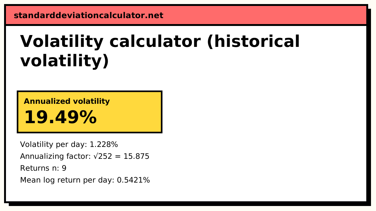
s = √0.000150735 = 0.0122774 = 1.228%
Scale by the square root of the number of periods in a year.
σannual = 0.0122774 × √252 = 19.49%
This is historical (realized) volatility, the sample standard deviation of past log returns. It is not implied volatility, which is backed out of option prices.
Using the volatility calculator
Paste prices oldest first, separated by commas, spaces or new lines; a column copied from a spreadsheet works. Set “Time between prices” to daily for closing prices on trading days, or weekly or monthly for those series. The headline is annualized volatility; the per-period figure is daily, weekly or monthly volatility to match.
How historical volatility is calculated
1. Log returns
rₜ = ln(Pₜ ÷ Pₜ₋₁)
n + 1 prices give n returns.
2. Standard deviation of returns
s = √( Σ(rₜ − r̄)² ÷ (n − 1) )
This is the sample standard deviation, dividing by n − 1. Some practitioners assume a mean return of zero for very short windows; with a few months of data or more the difference is small.
3. Annualizing with √252
σ(annual) = s × √k k = 252 daily, 52 weekly, 12 monthly
Variances of independent returns add, so the standard deviation grows with the square root of time. Hull’s Options, Futures, and Other Derivatives describes this way of estimating volatility from historical prices.
Worked example: ten closing prices
The calculator starts with ten daily closes:
100, 101.5, 100.8, 102.3, 103.1, 102, 103.8, 104.5, 103.2, 105
- Nine log returns (%): 1.4889, −0.6920, 1.4771, 0.7790, −1.0727, 1.7493, 0.6721, −1.2518, 1.7291. The first is ln(101.5 ÷ 100) = 0.014889.
- Mean: the log returns sum to ln(105 ÷ 100) = 0.048790, so r̄ = 0.048790 ÷ 9 = 0.0054211.
- Squared deviations sum to 0.00120588; divided by 8 that is a variance of 0.000150735.
- Daily volatility: √0.000150735 = 0.012277, or 1.228% a day.
- Annualized: 0.012277 × √252 = 0.012277 × 15.875 = 19.49%.
Simple vs log returns
A simple return is Pₜ ÷ Pₜ₋₁ − 1; a log return is ln(Pₜ ÷ Pₜ₋₁). For small moves they are almost equal: a 1.5% simple return is a 1.4889% log return. Log returns are preferred for volatility because they add across periods (the log returns above sum to the log return from the first price to the last), they treat a rise and the fall that undoes it symmetrically, and option pricing models assume log-normal prices. On the example, simple returns give an annualized volatility of 19.54% against 19.49% from log returns. The gap widens for assets with large daily moves.
Volatility and diversification
Volatility is the standard deviation of returns, so the rules for combining standard deviations apply. Two assets that are not perfectly correlated make a portfolio whose volatility is below the weighted average of theirs; the portfolio standard deviation calculator works it out. The article on volatility and diversification walks through why, and the guide to standard deviation in finance covers the other places the SD appears, from the Sharpe ratio to Bollinger Bands.
Common questions
How is historical volatility calculated?
Turn the prices into log returns, ln(Pₜ ÷ Pₜ₋₁), take the sample standard deviation of those returns, and multiply by the square root of the number of periods in a year: √252 for daily closes, √52 for weekly and √12 for monthly.
Why multiply by √252?
There are about 252 trading days in a year. If daily returns are independent, their variances add, so the annual variance is 252 times the daily variance and the annual standard deviation is √252 ≈ 15.87 times the daily one.
Should I use log returns or simple returns?
Log returns are the usual choice for historical volatility: they add up across periods and match the assumptions of option pricing models. For daily moves of a few percent the two give almost the same answer; the calculator shows both so you can see the gap.
How many prices do I need?
At least 3 prices (2 returns) for the calculator to work, but an estimate from so few returns is very noisy. Twenty trading days (about a month) is a common short window, and 60 to 252 days a common longer one.
Is historical volatility the same as implied volatility?
No. Historical volatility describes how much the price actually varied in the past. Implied volatility is the figure that makes an option pricing model match the option’s market price, so it reflects what traders expect for the future.
Related calculators
-
Sharpe ratio calculator
Return per unit of volatility, annualized.
-
Stock beta calculator
The market-driven part of a stock’s risk.
-
Portfolio standard deviation
Combine two volatilities with their correlation.
-
Sample standard deviation
The n − 1 step behind volatility, with working.