Math
Financial mathematics calculator
The time value of money in one place: grow or discount a lump sum, value an annuity or a perpetuity, convert between nominal and effective rates, and find the NPV, IRR and payback of a list of cash flows. Choose a calculation and fill in the numbers.
For an annuity, leave blank to solve for the payment from a PV or FV.
The first value is at time 0 (an outlay is negative), then one per period.
┄ Continuous curve ━ Balance
Show the working, step by step
The relation between the four quantities:
FV = PV × (1 + r/m)^(m t)
Rate per period i = r/m = 0.06/12 = 0.005; number of periods N = m t = 12 × 10 = 120.
FV = 1000 × (1 + 0.005)^120 = 1000 × 1.8193967 = 1819.3967
The effective annual rate, (1 + r/m)^m − 1 = 6.1678%, is the rate that would give the same growth compounded once a year.
The formulas
Throughout, r is the nominal annual rate, m the number of compounding (or payment) periods a year, i = r/m the rate per period, t the time in years and N = m t the number of periods.
Lump sum: FV = PV × (1 + i)^N PV = FV × (1 + i)^−N Continuous: FV = PV × e^(r t) Ordinary annuity: PV = PMT × (1 − (1 + i)^−N) ÷ i FV = PMT × ((1 + i)^N − 1) ÷ i Annuity due: multiply either by (1 + i) Perpetuity: PV = PMT ÷ (i − g) (needs i > g) Effective rate: EAR = (1 + r/m)^m − 1 continuous: EAR = e^r − 1 Net present value: NPV = Σ CFₜ ÷ (1 + r)^t IRR: the r with NPV = 0
The annuity formulas are geometric series. The present value of N payments is PMT(v + v² + … + v^N) with v = 1/(1 + i), and summing that series gives the factor (1 − v^N) ÷ i. Let N go to infinity and v^N goes to zero, which leaves the perpetuity value PMT ÷ i.
A worked example
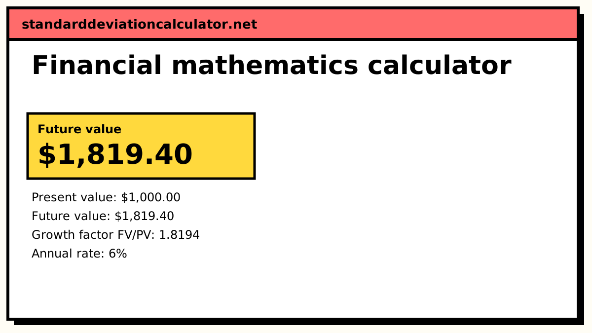
The calculator opens on a lump sum: $1,000 invested at 6% a year, compounded monthly, for 10 years, with the future value left blank so that it is the unknown.
- Rate per period: i = 0.06 ÷ 12 = 0.005. Number of periods: N = 12 × 10 = 120.
- Growth factor: 1.005^120 = 1.8194.
- Future value: 1,000 × 1.8194 = $1,819.40.
- The effective annual rate is 1.005^12 − 1 = 6.1678%, slightly above the nominal 6%.
Fill in the future value and clear a different box to solve for that one instead. With $2,000 as the target and the time left blank, the money takes 11.58 years to double. Clear the rate instead and the answer is the rate that gets from the present value to the future value in the time given.
Annuity and cash-flow examples
Switch to “Annuity” with the defaults: $200 a month for 10 years at 6%. The present-value factor is 90.0735 and the future-value factor 163.8793, so the payments are worth $18,014.69 today and $32,775.87 at the end. Paid at the start of each month (an annuity due), they are worth $18,104.76 and $32,939.75. Leave the payment blank and enter a future value of $50,000 to find the monthly payment that reaches it: $305.10.
The cash-flow default is an outlay of 10,000 followed by 3,000, 4,200 and 6,800. At 10% the present values are 2,727.27, 3,471.07 and 5,108.94, so the NPV is 1,307.29. The IRR, where the NPV falls to zero, is 16.34%. The running total reaches zero 2.41 periods in, and 2.74 periods in once each flow is discounted.
How compounding frequency changes the result
$1,000 at a nominal 6% a year for 10 years:
| Compounding | m | Effective annual rate | Value after 10 years |
|---|---|---|---|
| Annually | 1 | 6.0000% | $1,790.85 |
| Half-yearly | 2 | 6.0900% | $1,806.11 |
| Quarterly | 4 | 6.1364% | $1,814.02 |
| Monthly | 12 | 6.1678% | $1,819.40 |
| Daily | 365 | 6.1831% | $1,822.03 |
| Continuously | ∞ | 6.1837% | $1,822.12 |
The effective rate rises with m but levels off at e^r − 1. Compare rates on their effective values: 6% compounded monthly and 6.1678% compounded annually are the same rate written two ways.
Common mistakes
- Mixing periods. The rate per period and the number of periods must use the same unit. Monthly payments need the monthly rate r/12 and N in months. Using the annual rate with monthly periods treats every month as a full year of interest.
- Getting the payment timing wrong. Rent paid in advance is an annuity due. Valuing it as an ordinary annuity understates it by a factor of (1 + i).
-
Putting the first cash flow at t = 1. In NPV the first value is at time 0 and
is not discounted. Spreadsheet
NPV()functions discount the first value in their range by one period, so the usual pattern is=NPV(rate, B2:B4) + B1. - Trusting the IRR when cash flows change sign more than once. The IRR may not be unique, or may not exist. The NPV at a stated rate is always well defined.
- A perpetuity with growth at or above the rate. PMT ÷ (i − g) only converges for i > g. Otherwise each later payment is worth at least as much today as the one before, and the sum is infinite.
For savings with regular deposits over time, see the compound interest calculator.
Common questions
What is the difference between an ordinary annuity and an annuity due?
The timing of the payments. An ordinary annuity pays at the end of each period (loan repayments, most bond coupons); an annuity due pays at the start (rent, insurance premiums, many savings plans). Every payment of an annuity due arrives one period earlier, so it is worth exactly (1 + i) times as much. At 0.5% a month, 120 monthly payments of $200 have a present value of $18,014.69 as an ordinary annuity and $18,104.76 as an annuity due.
How do I convert a nominal rate to an effective annual rate?
Use EAR = (1 + r/m)^m − 1, where r is the nominal annual rate and m the number
of compounding periods a year. A 12% nominal rate compounded monthly is (1.01)^12 − 1 =
12.6825% effective. To go the other way, r = m × ((1 + EAR)^(1/m) − 1): an
effective 8% corresponds to a nominal 7.7208% compounded monthly.
Why can a project have more than one IRR?
The IRR is a root of a polynomial in 1/(1 + r), and a polynomial can have several roots. By Descartes' rule of signs, the number of IRRs above −100% is at most the number of changes of sign in the cash flows. The flows −100, +230, −132 change sign twice, and the NPV is zero at both 10% and 20%. When that happens the IRR does not rank projects reliably; use the NPV at your required rate instead. The calculator lists every IRR it finds between −99% and +1,000%.
How is the IRR calculated?
There is no closed-form formula for four or more cash flows, so it has to be found numerically. This calculator scans the NPV over a grid of rates to find where it changes sign, which gives a bracket that must contain a root. It then applies Newton's method inside that bracket and switches to bisection whenever a Newton step would jump outside it. The bracket guarantees convergence and Newton's method makes it fast. Spreadsheet IRR functions use Newton's method from a guess, which can fail or land on a different root.
What is the difference between the payback period and the discounted payback period?
The payback period counts how long the undiscounted cash flows take to repay the outlay. The discounted payback does the same with each flow converted to present value first, so it is always at least as long. For −10,000, 3,000, 4,200 and 6,800 at 10%, the payback is 2.41 periods and the discounted payback is 2.74. Neither looks at flows after the payback point, which is why NPV is the better measure of value.
Is continuous compounding much better than daily compounding?
Barely. At a nominal 6% the effective annual rate is 6.1831% with daily compounding and 6.1837% with continuous compounding (e^0.06 − 1). The step that matters is from annual to monthly compounding. Continuous compounding is used mainly because e^(rt) is easier to work with algebraically, for example in option pricing.
Related calculators
-
Compound interest
Savings growth with regular deposits, year by year.
-
Econometrics calculator
Elasticities, CAGR, GDP deflator and simple OLS.
-
Geometric mean
The average compound growth rate from a list of returns.
-
Sequences and series
Geometric series, the maths behind every annuity formula.