Math
Econometrics calculator
The calculations that come up again and again in economics and introductory econometrics courses. Choose a calculation, enter your figures, and get the answer with the formula worked through step by step.
Good A is the good whose demand you are studying.
Leave one of the three blank.
Separate with commas, spaces or new lines.
Same order and length as x.
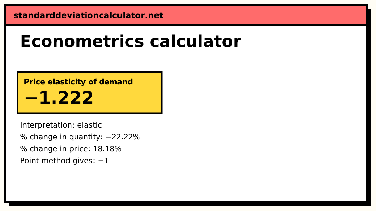
The price moves by 18.18% and the quantity by −22.22%; the elasticity is the ratio of the two. A flatter line means more elastic demand.
Show the working, step by step
Percentage change in quantity, measured from the average quantity:
base Q = (100 + 80) ÷ 2 = 90 %ΔQ = (80 − 100) ÷ 90 = −0.222222
Percentage change in price:
base P = (10 + 12) ÷ 2 = 11 %ΔP = (12 − 10) ÷ 11 = 0.181818
Divide the first by the second:
E = −0.222222 ÷ 0.181818 = −1.222
|E| > 1: demand is elastic, so price and total revenue move in opposite directions. Price elasticity of demand is negative for almost every good; many textbooks quote its absolute value.
Price elasticity of demand
point: E = (ΔQ ÷ Q₁) ÷ (ΔP ÷ P₁) midpoint: E = [ΔQ ÷ ((Q₁ + Q₂) ÷ 2)] ÷ [ΔP ÷ ((P₁ + P₂) ÷ 2)]
Elasticity measures how strongly quantity demanded responds to price, in percentage terms, so it does not depend on the units. The point method uses the starting values as the base. The midpoint (arc) method uses the averages, so the answer is the same whether the price rises or falls between the two values.
A worked example
The calculator's default: the price rises from 10 to 12 and quantity demanded falls from 100 to 80.
- Average quantity = (100 + 80) ÷ 2 = 90, so %ΔQ = −20 ÷ 90 = −22.22%.
- Average price = (10 + 12) ÷ 2 = 11, so %ΔP = 2 ÷ 11 = 18.18%.
- E = −22.22% ÷ 18.18% = −1.222. |E| > 1, so demand is elastic.
- Check with revenue: total revenue falls from 10 × 100 = 1,000 to 12 × 80 = 960. With elastic demand a price rise always cuts revenue.
The point method gives −20% ÷ 20% = −1 for the same data, which shows how much the base matters over a large change.
Income and cross-price elasticity
The same formula with income, or the price of another good, in place of the price. The sign tells you the type of good:
| Measure | Value | Meaning |
|---|---|---|
| Price elasticity | |E| > 1 / < 1 | Elastic / inelastic demand |
| Income elasticity | < 0 | Inferior good |
| Income elasticity | 0 to 1 | Normal good, necessity |
| Income elasticity | > 1 | Normal good, luxury |
| Cross elasticity | > 0 | Substitutes |
| Cross elasticity | < 0 | Complements |
In the default income example, income rises from 40,000 to 50,000 and quantity from 20 to 26: the midpoint income elasticity is 26.09% ÷ 22.22% = 1.174, a luxury. In the cross example the price of good B rises from 4 to 5 and sales of good A rise from 50 to 60, giving +0.818: substitutes.
GDP deflator and CAGR
GDP deflator = nominal GDP ÷ real GDP × 100 CAGR = (end ÷ start)^(1/n) − 1
Nominal GDP of 26,000 against real GDP of 21,500 gives a deflator of 120.93: prices are 20.93% above the base year. CAGR is the geometric-mean growth rate. A value growing from 5,000 to 8,000 over 6 years has a CAGR of 1.6^(1/6) − 1 = 8.15%.
Durbin–Watson statistic
d = Σₜ₌₂ (eₜ − eₜ₋₁)² ÷ Σₜ₌₁ eₜ² d ≈ 2(1 − ρ̂)
Enter the residuals from a time-series regression in time order. For the ten default residuals Σ(eₜ − eₜ₋₁)² = 5.64 and Σeₜ² = 7.08, so d = 0.797 and ρ̂ ≈ 0.60: consecutive residuals move together, a sign of positive autocorrelation. The test is only valid for a regression with an intercept and no lagged dependent variable among the regressors (use Durbin's h or the Breusch–Godfrey test then).
Simple OLS
β₁ = Sxy ÷ Sxx β₀ = ȳ − β₁x̄ SE(β₁) = s ÷ √Sxx s = √(SSE ÷ (n − 2))
For the eight default pairs the fitted line is ŷ = 9.9235 + 2.7602x, with SE(β₁) = 0.0742, so t = 37.19 on 6 degrees of freedom. R² = 0.9957 and adjusted R² = 0.9950. The OLS output also reports the Durbin–Watson statistic of its own residuals, useful when x is time. The standard errors assume the errors have constant variance and are uncorrelated; if a residual plot fans out, or d is far from 2, they will be too small.
Common mistakes
- Mixing methods. The point and midpoint methods give different numbers for the same data; use the one your course asks for.
- Reading the slope as an elasticity. A demand slope ΔQ ÷ ΔP depends on units; elasticity multiplies it by P ÷ Q.
- Averaging growth rates arithmetically. Use CAGR, not total growth divided by the number of years.
- Trusting R² alone. Two trending time series can give a high R² with no real relationship; check the Durbin–Watson statistic.
Common questions
What is the difference between the point and midpoint methods of elasticity?
Both divide a percentage change in quantity by a percentage change in price. The point method measures the changes from the starting values; the midpoint (arc) method measures them from the averages of the two values. When the price rises from 10 to 12 and quantity falls from 100 to 80, the point method gives −20% ÷ 20% = −1, while the midpoint method gives −22.22% ÷ 18.18% = −1.222. Going back from 12 to 10 with the point method would give a different answer (+25% ÷ −16.67% = −1.5); the midpoint answer is the same in both directions, which is why exam questions usually ask for it.
Why is price elasticity of demand negative?
Because demand curves slope downwards: when the price goes up the quantity demanded goes down, so the two percentage changes have opposite signs. Many textbooks and exam boards drop the sign and talk about |E|. Demand is elastic when |E| > 1, inelastic when |E| < 1 and unit elastic when |E| = 1.
How do I calculate real GDP from nominal GDP?
Divide nominal GDP by the GDP deflator and multiply by 100:
real GDP = nominal GDP ÷ deflator × 100. With nominal GDP of 26,000 and a
deflator of 120.93, real GDP is 21,500 in base-year prices. Leave the real GDP box blank
above and enter the other two to have it done for you.
What is a good Durbin–Watson value?
Close to 2. The statistic is roughly 2(1 − ρ), where ρ is the correlation between consecutive residuals, so 2 means no first-order autocorrelation. Values well below 2 (the example's 0.797) point to positive autocorrelation, which is common in time series and makes OLS standard errors too small. For a formal test compare d with the tabulated bounds dL and dU for your sample size and number of regressors.
What is the difference between R² and adjusted R²?
R² is the share of the variation in y explained by the regression. It never falls when
you add a regressor, even a useless one. Adjusted R² charges for each extra parameter:
1 − (1 − R²)(n − 1) ÷ (n − k − 1), with k regressors. In the default example
R² = 0.9957 and adjusted R² = 0.9950. With several regressors, use the
multiple regression calculator.
How is CAGR different from average annual growth?
CAGR is the constant yearly rate that compounds the start value into the end value:
(end ÷ start)^(1/n) − 1. Growing from 5,000 to 8,000 over 6 years is 60% in
total, a simple average of 10% a year, but only 8.15% a year compounded. The simple average
overstates growth because it ignores compounding.
Related calculators
-
Linear regression
Least-squares line, correlation and prediction for one predictor.
-
Multiple regression
OLS with several regressors, coefficient tests and adjusted R².
-
Financial mathematics
Present and future value, annuities, NPV and IRR.
-
Geometric mean
The average growth rate behind CAGR.
-
Correlation coefficient
Pearson's r and its significance test.