Math
Biostatistics calculator
Most results in medical research start as a 2×2 table: test result against true condition, or exposure against outcome. Enter the four counts to get the measures that go in a paper, each with a confidence interval and the working behind it.
| Condition present | Condition absent | Total | |
|---|---|---|---|
| Test positive | a = 90 | b = 40 | 130 |
| Test negative | c = 10 | d = 860 | 870 |
| Total | 100 | 900 | 1000 |
| Measure | Formula | Value | 95% CI |
|---|---|---|---|
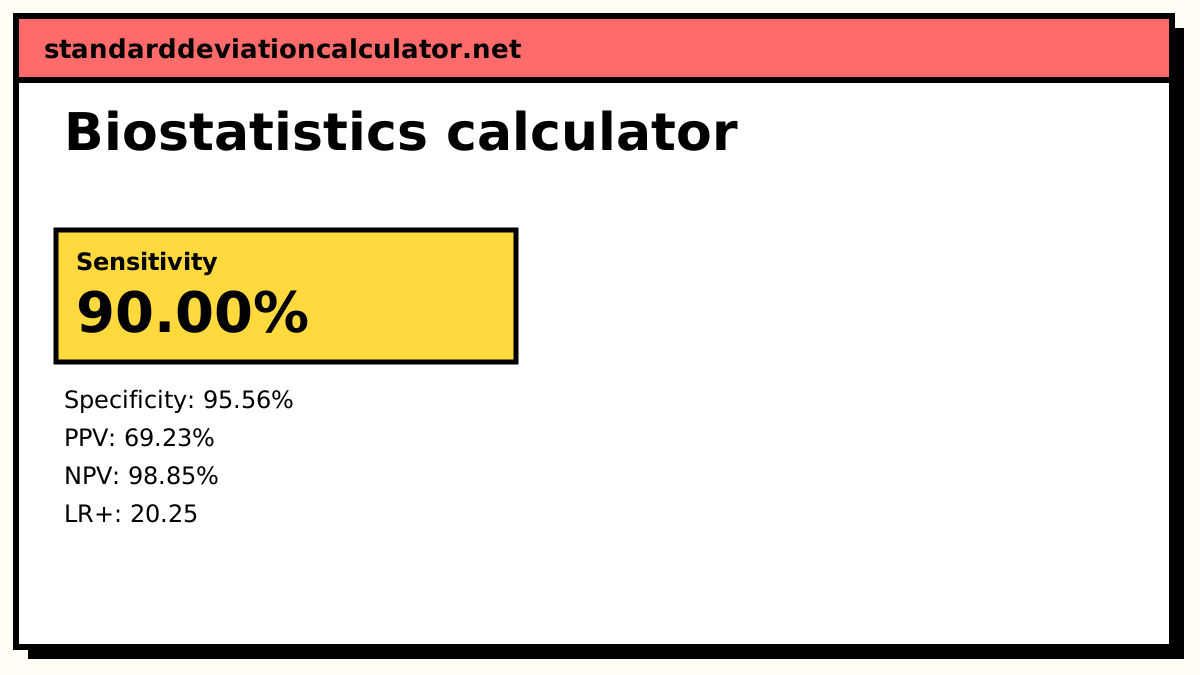
| Sensitivity | a ÷ (a + c) | 90.00% | 82.56% to 94.48% |
| Specificity | d ÷ (b + d) | 95.56% | 94.00% to 96.72% |
| Positive predictive value | a ÷ (a + b) | 69.23% | 60.84% to 76.52% |
| Negative predictive value | d ÷ (c + d) | 98.85% | 97.90% to 99.37% |
| Positive likelihood ratio | sens ÷ (1 − spec) | 20.25 | 14.85 to 27.61 |
| Negative likelihood ratio | (1 − sens) ÷ spec | 0.1047 | 0.05812 to 0.1884 |
| Diagnostic odds ratio | ad ÷ bc | 193.5 | 93.61 to 400 |
| Accuracy | (a + d) ÷ n | 95.00% | 93.47% to 96.19% |
| Prevalence | (a + c) ÷ n | 10.00% | 8.29% to 12.02% |
Show the working, step by step
Sensitivity: the share of people with the condition whom the test picks up.
sens = a ÷ (a + c) = 90 ÷ 100 = 90.00%
Specificity: the share of people without it whom the test clears.
spec = d ÷ (b + d) = 860 ÷ 900 = 95.56%
Predictive values read along the rows, so they depend on the prevalence in this sample.
PPV = a ÷ (a + b) = 90 ÷ 130 = 69.23% NPV = d ÷ (c + d) = 860 ÷ 870 = 98.85%
Likelihood ratios combine sensitivity and specificity and do not depend on prevalence.
LR+ = 0.9 ÷ (1 − 0.95556) = 20.25 LR− = (1 − 0.9) ÷ 0.95556 = 0.1047
Diagnostic odds ratio with a log (Woolf) interval, z = 1.96:
DOR = (90 × 860) ÷ (40 × 10) = 193.5 SE(ln DOR) = √(1/a + 1/b + 1/c + 1/d) = 0.3705 95% CI: exp(ln 193.5 ± 1.96 × 0.3705) = 93.61 to 400
Chi-square test of independence (1 degree of freedom):
χ² = n(ad − bc)² ÷ [(a+b)(c+d)(a+c)(b+d)] = 1000 × (90×860 − 40×10)² ÷ (130 × 870 × 100 × 900) = 582.47 p = < 0.0001 Fisher's exact p = < 0.0001
Proportions use Wilson score intervals; likelihood ratios and the odds ratio use log-method intervals.
The table layout
| Condition present / outcome | Condition absent / no outcome | |
|---|---|---|
| Test positive / exposed or treated | a | b |
| Test negative / unexposed or control | c | d |
Rows are the thing you know first (the test result, or whether someone was exposed or treated); columns are the truth or the outcome. Put your data in this orientation. Swapping the rows inverts the relative risk and odds ratio, and swapping the columns turns sensitivity into the false-negative rate.
Diagnostic test measures
sensitivity = a ÷ (a + c) specificity = d ÷ (b + d) PPV = a ÷ (a + b) NPV = d ÷ (c + d) LR+ = sens ÷ (1 − spec) LR− = (1 − sens) ÷ spec
The calculator's default is a screening test given to 1,000 people, 100 of whom have the condition. It picks up 90 of them (a = 90, c = 10) and wrongly flags 40 of the 900 who do not (b = 40, d = 860).
- Sensitivity = 90 ÷ 100 = 90.00%; specificity = 860 ÷ 900 = 95.56%.
- PPV = 90 ÷ 130 = 69.23%: nearly a third of positive results are false alarms.
- NPV = 860 ÷ 870 = 98.85%.
- LR+ = 0.9 ÷ (1 − 0.9556) = 20.25; LR− = 0.1 ÷ 0.9556 = 0.1047.
- Accuracy = (90 + 860) ÷ 1,000 = 95.00%, and the prevalence in the sample is 10.00%.
A likelihood ratio above 10 or below 0.1 usually changes a diagnosis. Multiply the pre-test odds by LR+ to get the post-test odds after a positive result: 0.1 ÷ 0.9 × 20.25 = 2.25, a probability of 2.25 ÷ 3.25 = 69.23%, the same as the PPV.
Measures of association
RR = [a ÷ (a + b)] ÷ [c ÷ (c + d)] OR = ad ÷ bc RD = a ÷ (a + b) − c ÷ (c + d) NNT = 1 ÷ |RD| 95% CI for RR or OR = exp(ln estimate ± 1.96 × SE)
Switch the table type to “Exposure or treatment × outcome” for the default trial: 15 of 100 treated patients and 30 of 100 controls had the outcome.
| Measure | Estimate | 95% CI |
|---|---|---|
| Relative risk | 0.5000 | 0.2872 to 0.8704 |
| Odds ratio | 0.4118 | 0.2053 to 0.8258 |
| Risk difference | −15.00% | −26.39% to −3.61% |
| Number needed to treat | 6.667 | 3.790 to 27.67 |
Treatment halves the risk (RR 0.5), an absolute reduction of 15 percentage points, so about 7 patients need treating to prevent one outcome. The chi-square statistic is 6.452 on 1 degree of freedom (p = 0.0111), and Fisher's exact p is 0.0171.
Reading the results
- An interval that includes 1 (for RR or OR) or 0 (for the risk difference) means the data are consistent with no effect at that confidence level.
- Relative and absolute effects answer different questions. A relative risk of 0.5 sounds the same whether the risk falls from 30% to 15% or from 0.2% to 0.1%, but the NNT is 7 in the first case and 1,000 in the second.
- Predictive values do not transfer. PPV and NPV from a study sample apply only to populations with the same prevalence. Sensitivity, specificity and likelihood ratios travel better.
- Zero cells. A zero makes the log interval undefined. The calculator then adds 0.5 to every cell for the odds ratio and relative risk and says so.
Common questions
What is the difference between sensitivity and positive predictive value?
Sensitivity reads down the “condition present” column: of the people who have the condition, what share test positive? In the default table that is 90 ÷ 100 = 90%. The positive predictive value reads across the “test positive” row: of the people who test positive, what share have the condition? That is 90 ÷ 130 = 69.23%. Sensitivity is a property of the test; PPV also depends on how common the condition is.
Why does the PPV fall when the condition is rare?
Because false positives come from the much larger group without the condition. Keep the default test (sensitivity 90%, specificity 95.56%) but drop the prevalence from 10% to 1%: out of 10,000 people, 90 of the 100 with the condition test positive, and 440 of the 9,900 without it do too. The PPV falls to 90 ÷ 530 = 16.98%. Likelihood ratios do not change with prevalence, which is why they are preferred for comparing tests.
When should I report an odds ratio instead of a relative risk?
Use the relative risk for cohort studies and trials, where you follow groups and count who develops the outcome. In a case-control study you choose people by outcome, so the row risks are not real risks and only the odds ratio is valid. When the outcome is rare (under about 10%), the odds ratio is close to the relative risk; for common outcomes it lies further from 1, as in the default trial (OR 0.41 against RR 0.50).
How is the 95% confidence interval for a relative risk calculated?
On the log scale, where the sampling distribution is close to normal:
SE(ln RR) = √(1/a − 1/(a+b) + 1/c − 1/(c+d)), and the interval is
exp(ln RR ± 1.96 × SE). For the default trial, SE = 0.2828 and the interval is
0.2872 to 0.8704. It excludes 1, so the reduction in risk is statistically significant at
the 5% level.
What does a number needed to treat of 6.67 mean?
On average, 6.67 people have to receive the treatment instead of the control for one extra person to avoid the outcome. It is 1 ÷ the absolute risk reduction (1 ÷ 0.15 here) and is rounded up to 7 when reported, since you cannot treat part of a person. If the treatment increases the risk, the same reciprocal is the number needed to harm.
Should I use the chi-square test or Fisher's exact test?
The chi-square p-value is an approximation that works when every expected count is at least 5. With smaller counts use Fisher's exact test, which the calculator also reports; it computes the probability of the table directly from the hypergeometric distribution. Yates' correction makes the chi-square more conservative on small tables but is often too cautious.
Related calculators
-
Chi-square calculator
Tests of independence and goodness of fit on larger tables.
-
Bayes' theorem
Turn prevalence, sensitivity and specificity into a post-test probability.
-
Confidence interval
Intervals for a mean or a proportion.
-
Sample size
How many participants a study needs for a given margin of error.
-
P-value calculator
P-values from z, t, chi-square and F statistics.