Math
Data analysis calculator: frequency distribution
Paste raw data and get a grouped frequency distribution: the class table with relative and cumulative frequencies, a histogram, both ogives, and the grouped mean, median and mode worked out step by step.
Separate values with commas, spaces or new lines.
Blank: a multiple of the width just below the smallest value (class width), or the smallest value itself (number of classes, Sturges).
| Class | Midpoint x | f | Relative f | Cum. f (less than) | Cum. f (more than) | f·x |
|---|---|---|---|---|---|---|
| 30–40 | 35 | 2 | 0.06667 | 2 | 30 | 70 |
| 40–50 | 45 | 5 | 0.1667 | 7 | 28 | 225 |
| 50–60 | 55 | 7 | 0.2333 | 14 | 23 | 385 |
| 60–70 | 65 | 9 | 0.3 | 23 | 16 | 585 |
| 70–80 | 75 | 4 | 0.1333 | 27 | 7 | 300 |
| 80–90 | 85 | 3 | 0.1 | 30 | 3 | 255 |
| Total | 30 | 1 | 1820 |
Exclusive classes: each class includes its lower limit and excludes its upper limit, so a value of exactly 40 goes in the second class.
Histogram
Ogives
━ “Less than” ogive ━ “More than” ogive
The two ogives cross at the median: half the observations lie below it and half above.
Show the working, step by step
Range and Sturges' rule.
range = 88 − 35 = 53 k = ⌈1 + log₂ 30⌉ = ⌈1 + 4.907⌉ = 6
Class width chosen: h = 10, first class from 30. That gives 6 classes to reach the largest value, 88.
k = ⌊(88 − 30) ÷ 10⌋ + 1 = 6
Count the values in each class (f), then accumulate them.
30–40: f = 2, cf = 2 40–50: f = 5, cf = 7 50–60: f = 7, cf = 14 60–70: f = 9, cf = 23 70–80: f = 4, cf = 27 80–90: f = 3, cf = 30
Grouped mean: multiply each midpoint by its frequency, add, divide by n.
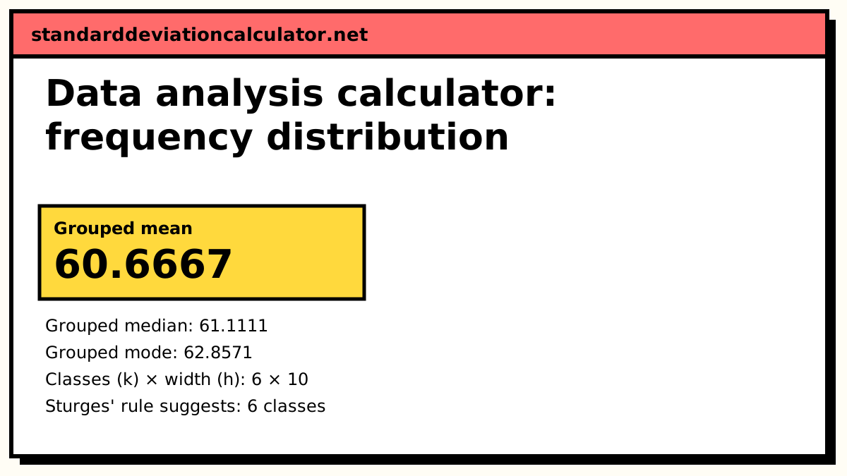
x̄ = Σf·x ÷ n = 1820 ÷ 30 = 60.6667
Grouped median: n ÷ 2 = 15, and the first class with cf ≥ 15 is 60–70. Use l = 60, cf before = 14, f = 9, h = 10.
median = l + ((n/2 − cf) ÷ f) × h = 60 + ((15 − 14) ÷ 9) × 10 = 61.1111
Grouped mode: the modal class is 60–70 (f₁ = 9), with f₀ = 7 before it and f₂ = 4 after it.
mode = l + ((f₁ − f₀) ÷ (2f₁ − f₀ − f₂)) × h = 60 + ((9 − 7) ÷ (18 − 7 − 4)) × 10 = 62.8571
Grouped values are estimates: they assume the values in each class are spread evenly across it. The raw data give mean 60.7333 and median 60.5.
How the classes are chosen
A frequency distribution sorts n values into k classes of equal width h. You can fix the width yourself, fix the number of classes, or let Sturges’ rule pick k:
k = ⌈1 + log₂ n⌉ h = range ÷ k, rounded up to the data’s unit
When you choose k (directly or by Sturges), the width is the smallest multiple of the data’s recording unit (1 for whole numbers, 0.1 for one decimal place) with k × h greater than the range, and the first class starts at the smallest value. That guarantees exactly k classes, with the maximum inside the last one. When you choose the width, the first class starts at the multiple of h just below the minimum, so classes line up on round numbers. You can override the start in either case.
The grouped formulas
mean x̄ = Σ f·x ÷ n median = l + ((n/2 − cf) ÷ f) × h mode = l + ((f₁ − f₀) ÷ (2f₁ − f₀ − f₂)) × h
Here x is a class midpoint, l the lower boundary of the median (or modal) class, cf the cumulative frequency of the classes before the median class, f the median class’s frequency, f₁ the modal class’s frequency, and f₀ and f₂ the frequencies of the classes either side of it (0 at the ends of the table).
A worked example
The default data are 30 exam marks, from 35 to 88 (range 53). Sturges gives k = ⌈1 + log₂ 30⌉ = ⌈5.907⌉ = 6, and a width of 10 starting at 30 also gives six classes:
| Class | Midpoint | f | Relative f | Less-than cf | More-than cf |
|---|---|---|---|---|---|
| 30–40 | 35 | 2 | 0.0667 | 2 | 30 |
| 40–50 | 45 | 5 | 0.1667 | 7 | 28 |
| 50–60 | 55 | 7 | 0.2333 | 14 | 23 |
| 60–70 | 65 | 9 | 0.3000 | 23 | 16 |
| 70–80 | 75 | 4 | 0.1333 | 27 | 7 |
| 80–90 | 85 | 3 | 0.1000 | 30 | 3 |
- Mean: Σ f·x = 1,820, so x̄ = 1,820 ÷ 30 = 60.67.
- Median: n ÷ 2 = 15. The cumulative frequency passes 15 in 60–70 (cf before = 14, f = 9), so median = 60 + ((15 − 14) ÷ 9) × 10 = 61.11.
- Mode: the modal class is 60–70 with f₁ = 9, f₀ = 7, f₂ = 4, so mode = 60 + (2 ÷ 7) × 10 = 62.86.
The raw marks have mean 60.73 and median 60.5, close to the grouped estimates. Switch the calculator to Sturges’ rule and it uses width ⌈53 ÷ 6⌉ = 9 from 35 instead (35–44, 44–53 and so on), which moves the grouped mean to 61.4 and the mode to 59.75: grouped statistics depend on where the class limits fall.
Reading the ogives
The “less than” ogive plots each upper boundary against the number of values below it, rising from 0 to n. The “more than” ogive plots each lower boundary against the number of values at or above it, falling from n to 0. They cross at the median. Read any other percentile from the less-than ogive: the first quartile sits where it passes n ÷ 4.
Common mistakes
- Using stated limits of inclusive classes in the formulas. For 30–39 the lower boundary is 29.5, not 30. Using 30 shifts every grouped median and mode up by half a unit.
- Unequal or overlapping classes. A value of 40 cannot belong to both 30–40 and 40–50. Exclusive classes put it in the upper one; this tool follows that convention.
- Too many or too few classes. With 5 classes for 1,000 values the shape disappears; with 40 classes for 30 values most classes hold 0 or 1. Sturges’ rule is a sensible middle, and the histogram shows at a glance whether the grouping works.
- Treating grouped statistics as exact. They are estimates. For the exact mean, standard deviation and quartiles of raw data, use the descriptive statistics calculator.
Common questions
What is Sturges’ rule for the number of classes?
k = ⌈1 + log₂ n⌉, often written 1 + 3.322 log₁₀ n. It
suggests 6 classes for 30 values, 7 for 50, 8 for 100 and 11 for 1,000. Divide the range by
k and round up to get the class width. It was designed for roughly bell-shaped data and gives
too few classes for large or skewed samples, so treat it as a starting point.
What is the difference between inclusive and exclusive classes?
Exclusive classes share their limits (30–40, 40–50): each class includes its lower limit and excludes the upper one, so 40 goes in 40–50. Inclusive classes do not overlap (30–39, 40–49) and suit whole-number data. For grouped calculations an inclusive class is widened to its true boundaries, 29.5–39.5, which is why its midpoint is 34.5 rather than 35.
How do you find the median from an ogive?
Draw the “less than” ogive (cumulative frequency against upper class boundary), go across from n ÷ 2 on the vertical axis to the curve, and read the value below. Or draw both ogives: they cross at the median. For the default data both methods give 61.11, the same as the grouped median formula, because the ogive joins its points with straight lines.
Why are the grouped mean and median different from the raw values?
Grouping throws away the exact values. The grouped mean treats every value as sitting at its class midpoint, and the median formula assumes values are spread evenly inside the median class. For the default data the grouped mean is 60.67 against a true mean of 60.73. If you have the raw data, report the raw statistics and use the table for the picture.
What does relative frequency tell you?
The share of all observations in a class: f ÷ n. The relative frequencies add to 1 (or 100%), so two data sets of different sizes can be compared class by class. In the default table 9 of 30 marks fall in 60–70, a relative frequency of 0.30.
Related calculators
-
Descriptive statistics
The full numeric summary of raw data: mean, SD, quartiles, skewness.
-
Histogram maker
Draw a histogram straight from a list of numbers.
-
Grouped data standard deviation
Mean, variance and SD from a frequency table.
-
Mean, median and mode
The three averages of ungrouped data.
-
Quartile calculator
Q1, Q2 and Q3 with the working.