Frequency distribution calculator
Paste raw data to build a frequency distribution table. Choose grouped classes or one row per value, and the calculator fills in every column from f to cumulative relative frequency.
Numbers, or words such as survey answers (words give an ungrouped table).
| Class | Boundaries | Midpoint | f | Relative f | Percent | Cumulative f | Cum. relative f |
|---|---|---|---|---|---|---|---|
| 23–28 | 22.5–28.5 | 25.5 | 4 | 0.1667 | 16.67% | 4 | 0.1667 |
| 29–34 | 28.5–34.5 | 31.5 | 5 | 0.2083 | 20.83% | 9 | 0.375 |
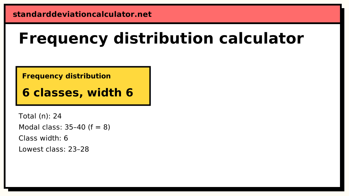
| 35–40 | 34.5–40.5 | 37.5 | 8 | 0.3333 | 33.33% | 17 | 0.7083 |
| 41–46 | 40.5–46.5 | 43.5 | 4 | 0.1667 | 16.67% | 21 | 0.875 |
| 47–52 | 46.5–52.5 | 49.5 | 2 | 0.08333 | 8.333% | 23 | 0.9583 |
| 53–58 | 52.5–58.5 | 55.5 | 1 | 0.04167 | 4.167% | 24 | 1 |
| Total | 24 | 1 | 100% |
Show the working, step by step
Choose the classes.
k = ⌈1 + log₂ 24⌉ = ⌈5.585⌉ = 6; raw width = range ÷ k = 31 ÷ 6 = 5.16667 round up to the data’s precision (1), adding a unit if it is already exact: width = 6 classes: 23–28, 29–34, 35–40, 41–46, 47–52, 53–58
Tally the values into classes to get each frequency f.
23–28: 4, 29–34: 5, 35–40: 8, 41–46: 4, 47–52: 2, 53–58: 1
Relative frequency = f ÷ n.
23–28: 4 ÷ 24 = 0.1667
Cumulative frequency is the running total of f; divide it by n for the cumulative relative frequency.
4, 9, 17, 21, 23, 24 → last = n = 24
Boundaries sit half a unit outside the class limits so that the classes meet without gaps.
The columns
relative frequency = f ÷ n cumulative frequency (cf) = f₁ + f₂ + … + f (up to this class) cumulative relative frequency = cf ÷ n midpoint = (lower limit + upper limit) ÷ 2
The frequencies add to n, the relative frequencies add to 1, and the last cumulative frequency equals n. Those three checks catch most tallying mistakes.
A worked example
The default data is the ages of 24 people in a fitness class:
23, 25, 27, 28, 30, 31, 31, 33, 34, 35, 35, 36, 37, 38, 38, 39, 40, 42, 43, 45, 46, 48, 51, 54
Sturges' rule gives k = ⌈1 + log₂ 24⌉ = ⌈5.585⌉ = 6 classes. The range is 54 − 23 = 31, and 31 ÷ 6 = 5.17 rounds up to a class width of 6. Starting at the minimum, 23, the classes are:
| Class | Boundaries | Midpoint | f | Relative f | cf | Cum. rel. f |
|---|---|---|---|---|---|---|
| 23–28 | 22.5–28.5 | 25.5 | 4 | 0.1667 | 4 | 0.1667 |
| 29–34 | 28.5–34.5 | 31.5 | 5 | 0.2083 | 9 | 0.375 |
| 35–40 | 34.5–40.5 | 37.5 | 8 | 0.3333 | 17 | 0.7083 |
| 41–46 | 40.5–46.5 | 43.5 | 4 | 0.1667 | 21 | 0.875 |
| 47–52 | 46.5–52.5 | 49.5 | 2 | 0.0833 | 23 | 0.9583 |
| 53–58 | 52.5–58.5 | 55.5 | 1 | 0.0417 | 24 | 1 |
For the first class, the relative frequency is 4 ÷ 24 = 0.1667. The cumulative frequency of the third class is 4 + 5 + 8 = 17, and 17 ÷ 24 = 0.7083.
Interpreting the table
The modal class is 35–40, which holds a third of the group. From the cumulative columns, 9 people (37.5%) are 34 or younger and 21 people (87.5%) are 46 or younger. The frequencies fall off more slowly above the modal class than below it, with the oldest class holding a single person, so the ages lean slightly to the right.
The midpoints are what you use to estimate the mean or standard deviation from grouped data: each class is treated as if all its values sat at the midpoint. Here that estimate of the mean is (4 × 25.5 + 5 × 31.5 + 8 × 37.5 + 4 × 43.5 + 2 × 49.5 + 1 × 55.5) ÷ 24 = 37, close to the true mean of the raw ages, 37.04.
Choosing your own classes
Rules like Sturges' give a sensible starting point, but round class limits are easier to read. Choose “Class width I choose”, type 5, and set the first class to start at 20. The same ages then fall into seven classes: 20–24 (1), 25–29 (3), 30–34 (5), 35–39 (7), 40–44 (3), 45–49 (3) and 50–54 (2). The modal class moves to 35–39, and the table still adds to 24. Whatever classes you choose, they must not overlap, must have the same width, and must cover every value from the minimum to the maximum.
Common mistakes
- Overlapping classes such as 23–29 and 29–35, which count the value 29 twice.
- Classes of unequal width without saying so; the frequencies are then not comparable.
- Treating boundaries and limits as the same thing. Limits are the values in the table; boundaries lie half a unit outside them.
- Forgetting to check that the frequencies add up to n.
Common questions
What is a frequency distribution?
A table that shows how often each value, or each range of values, occurs in a data set. The basic column is the frequency f. Relative frequency (f ÷ n) turns counts into shares, and the cumulative columns give running totals: how many values, or what fraction, fall at or below each class.
Should I use a grouped or an ungrouped table?
Ungrouped (one row per value) when there are only a few distinct values, such as the number of children per family, dice rolls or survey answers. Grouped (one row per class) when the values are spread out or continuous, such as ages, heights or times, where an ungrouped table would have almost every count equal to 1.
How do I find the number of classes and the class width?
A common choice is Sturges' rule, k = ⌈1 + log₂ n⌉. The class width is then the range divided by k, rounded up. For 24 values from 23 to 54 that gives k = 6 and 31 ÷ 6 = 5.17, rounded up to 6. You can also type your own number of classes or class width.
What does the cumulative relative frequency tell me?
The fraction of the data at or below the upper boundary of a class. In the example, the cumulative relative frequency of the 35–40 class is 0.7083, so about 71% of the people are 40 or younger. It always ends at 1, and it is what an ogive (cumulative frequency graph) plots.
Can I make a frequency table of words?
Yes. If the data contains words, the calculator counts each distinct answer and lists them in the order they first appear. The cumulative columns are still shown but only mean something if the categories have a natural order, such as ratings from “poor” to “excellent”.
Related calculators
-
SD from a frequency table
Mean and standard deviation from values and their frequencies.
-
Grouped data SD
Mean and standard deviation from class intervals.
-
Relative frequency
Shares of the total for each value or category.