Histogram calculator
Paste raw data and pick a rule for the bins. The calculator works out the class width, tallies a frequency table and draws the histogram, showing each step.
Raw data, separated by commas, spaces or new lines.
Leave blank to start at the smallest value. It must not be above the minimum.
Bars run between class boundaries (half a unit outside the class limits), so neighbouring bars touch.
| Class | Boundaries | Midpoint | f | Relative f | Cumulative f |
|---|---|---|---|---|---|
| 12–19 | 11.5–19.5 | 15.5 | 4 | 0.16 | 4 |
| 20–27 | 19.5–27.5 | 23.5 | 7 | 0.28 | 11 |
| 28–35 | 27.5–35.5 | 31.5 | 7 | 0.28 | 18 |
| 36–43 | 35.5–43.5 | 39.5 | 3 | 0.12 | 21 |
| 44–51 | 43.5–51.5 | 47.5 | 2 | 0.08 | 23 |
| 52–59 | 51.5–59.5 | 55.5 | 2 | 0.08 | 25 |
| Total | 25 | 1 |
Show the working, step by step
Find the range.
range = 58 − 12 = 46
Class width by Sturges’ rule:
k = ⌈1 + log₂ 25⌉ = ⌈5.644⌉ = 6; raw width = range ÷ k = 46 ÷ 6 = 7.66667 round up to the data’s precision (1), adding a unit if it is already exact: width = 8
Start the first class at 12 and add the width until the maximum is covered.
12–19, 20–27, 28–35, 36–43, 44–51, 52–59
Tally each value into its class and draw a bar of that height from boundary to boundary.
12–19: 4, 20–27: 7, 28–35: 7, 36–43: 3, 44–51: 2, 52–59: 2
Each class includes its lower limit and stops just below the next class’s lower limit.
The binning rules
Sturges: k = ⌈1 + log₂ n⌉ Square root: k = ⌈√n⌉ Rice: k = ⌈2 ∛n⌉ Scott: h = 3.49 s n^(−1/3) Freedman–Diaconis: h = 2 × IQR × n^(−1/3)
The first three give a number of classes k, and the width is the range divided by k. The last two give a width h directly, from the standard deviation s or the interquartile range. Either way the width is then rounded up to the precision of the data, and classes are added from the starting point until the maximum is covered.
A worked example
The default data is 25 commute times in minutes:
12, 15, 17, 18, 21, 22, 22, 24, 25, 26, 27, 28, 29, 30, 31, 33, 34, 35, 36, 38, 41, 44, 47, 52, 58
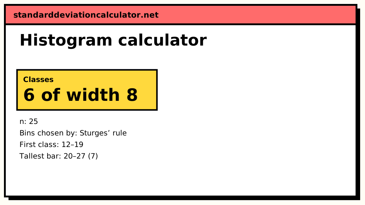
The range is 58 − 12 = 46. Sturges' rule gives k = ⌈1 + log₂ 25⌉ = ⌈5.644⌉ = 6 classes, and a raw width of 46 ÷ 6 = 7.67, which rounds up to 8. Starting at the minimum, 12:
| Class | Boundaries | f | Relative f |
|---|---|---|---|
| 12–19 | 11.5–19.5 | 4 | 0.16 |
| 20–27 | 19.5–27.5 | 7 | 0.28 |
| 28–35 | 27.5–35.5 | 7 | 0.28 |
| 36–43 | 35.5–43.5 | 3 | 0.12 |
| 44–51 | 43.5–51.5 | 2 | 0.08 |
| 52–59 | 51.5–59.5 | 2 | 0.08 |
The Rice rule also gives 6 classes here. The square-root rule gives k = 5 and a width of 10 (46 ÷ 5 = 9.2, rounded up). Freedman–Diaconis uses the IQR, 36 − 22 = 14, to get h = 2 × 14 ÷ ∛25 = 9.58, so it also lands on a width of 10. Scott's rule, with s = 11.51, gives h = 13.73 and only four wide classes of 14.
Reading the histogram
The tallest bars are the 20–27 and 28–35 minute classes, which together hold 14 of the 25 commutes. To the right the bars step down slowly through 36–43, 44–51 and 52–59, while on the left there is only one class. That long right tail means the distribution is right-skewed, which is common for times and incomes: there is a floor on how short a commute can be but no hard ceiling. The mean, 30.6 minutes, is pulled toward the tail and sits above the median of 29 minutes.
Try the other rules to see how much the picture depends on the bins. With four classes Scott's rule hides the right tail almost completely. If a feature appears only for one bin width, be careful about reading too much into it.
Common mistakes
- Leaving gaps between bars. For continuous data the bars run from boundary to boundary and touch.
- Using unequal class widths and plotting raw frequencies; wider classes then look more important than they are.
- Rounding the width down, which leaves the maximum outside every class.
- Counting a value on a class edge in both classes, so the frequencies add to more than n.
Common questions
How many bins should a histogram have?
There is no single right answer, which is why several rules exist. Sturges' rule, k = ⌈1 + log₂ n⌉, is the classic default and suits small, roughly bell-shaped data. The square-root rule is quick to do by hand. Scott's and the Freedman–Diaconis rules choose a width from the spread of the data and work better for large samples; Freedman–Diaconis uses the IQR, so outliers do not inflate it. Most textbook exercises use between 5 and 20 classes.
Why is the width rounded up instead of rounded normally?
Rounding down can leave the largest value outside the last class. Rounding up to the data's precision (a whole number for whole-number data) guarantees the classes reach the maximum. When the raw width is already a whole number, the calculator adds one unit, because k classes of exactly that width starting at the minimum would stop one unit short.
What is the difference between class limits and class boundaries?
Limits are the values written in the table, such as 12–19 and 20–27. There is a gap of one unit between 19 and 20, so the bars are drawn between the boundaries, 11.5–19.5 and 19.5–27.5, which sit half a unit outside the limits. That is why the bars of a histogram touch.
Which class does a value on the edge go into?
Here each class includes its lower limit and stops just below the next lower limit. With whole numbers and classes 12–19 and 20–27, the value 20 goes in the second class. State the rule you use, because software differs on it.
How is a histogram different from a bar chart?
A histogram shows a continuous numeric variable divided into intervals, so the bars touch and the horizontal axis is a number line. A bar chart shows separate categories, so the bars have gaps and their order can be changed without changing the meaning.
Related calculators
-
Histogram maker
A histogram with a fitted normal curve and the standard deviation.
-
Class width calculator
Class width, limits and boundaries step by step.
-
Frequency distribution
Full grouped table with cumulative and relative frequencies.