Sharpe ratio calculator
The Sharpe ratio measures return per unit of risk: the average return above a risk-free rate, divided by the standard deviation of returns. Paste a list of periodic returns, or enter a mean return and standard deviation you already have, pick the return period and the calculator gives the per-period and annualized ratio with each step.
One return per period in percent (2.1 = 2.1%), oldest first. At least 2.
Divided by the periods per year to get the per-period rate.
| Period | Return r | r − r̄ | (r − r̄)² |
|---|---|---|---|
| 1 | 2.1% | 1.125% | 1.266 |
| 2 | −1.3% | −2.275% | 5.176 |
| 3 | 3.4% | 2.425% | 5.881 |
| 4 | 0.8% | −0.175% | 0.03063 |
| 5 | −0.5% | −1.475% | 2.176 |
| 6 | 1.9% | 0.925% | 0.8556 |
| 7 | 2.7% | 1.725% | 2.976 |
| 8 | −2.2% | −3.175% | 10.08 |
| 9 | 1.5% | 0.525% | 0.2756 |
| 10 | 0.6% | −0.375% | 0.1406 |
| 11 | 3.1% | 2.125% | 4.516 |
| 12 | −0.4% | −1.375% | 1.891 |
Show the working, step by step
Average the returns.
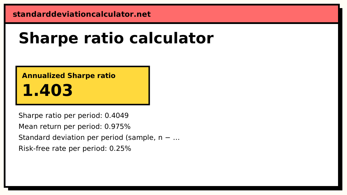
r̄ = Σr ÷ 12 = 0.975%
Sum the squared deviations from the mean and divide by n − 1 (sample standard deviation).
Σ(r − r̄)² = 35.2625 (%²) s = √(35.2625 ÷ 11) = 1.7904%
Convert the annual risk-free rate to the period.
Rf = 3% ÷ 12 = 0.25%
Divide the excess return by the standard deviation.
S = (0.975% − 0.25%) ÷ 1.7904% = 0.4049
Annualize by multiplying by the square root of the periods per year.
Sannual = 0.4049 × √12 = 1.403
The √-of-time rule assumes returns are independent from one period to the next. Compare Sharpe ratios only when they use the same return frequency, period and risk-free rate.
Two ways to use the Sharpe ratio calculator
From a return series. Enter one return per period in percent, oldest first, such as twelve monthly returns from a fund factsheet or a spreadsheet column. The calculator finds the mean and the sample standard deviation itself and shows the table of deviations.
From mean, SD and risk-free rate. If you already have the average return and the standard deviation for one period, switch “Start from” and enter them directly. They are used as entered; nothing is recomputed.
In both modes the risk-free rate is entered as an annual rate and divided by the number of periods in a year (3% a year is 0.25% a month). Some analysts compound instead, (1 + Rf)1/12 − 1; at ordinary interest rates the two differ in the third decimal place of the ratio.
The Sharpe ratio formula
S = (R̄p − Rf) ÷ σp
R̄p is the mean return of the portfolio over the period, Rf the risk-free return for the same period and σp the standard deviation of the portfolio’s returns. The numerator is the excess return; the denominator is the risk taken to earn it. William Sharpe set out the ratio in this excess-return form in “The Sharpe Ratio” (Journal of Portfolio Management, 1994).
The standard deviation is where most of the work is. This calculator uses the sample standard deviation, which divides the sum of squared deviations by n − 1:
σp = √( Σ(r − r̄)² ÷ (n − 1) )
Strictly, Sharpe’s definition uses the standard deviation of the excess returns r − Rf. With a constant risk-free rate, as here, subtracting it from every return does not change the spread, so the two are the same number.
Annualizing a Sharpe ratio
A mean return grows in proportion to time, while a standard deviation grows with the square root of time when returns are independent. So a per-period Sharpe ratio is annualized by multiplying by the square root of the number of periods in a year:
S(annual) = S(period) × √k k = 252 daily, 52 weekly, 12 monthly, 1 annual
Worked example: twelve monthly returns
The calculator starts with these monthly returns (%) and a 3% annual risk-free rate:
2.1, −1.3, 3.4, 0.8, −0.5, 1.9, 2.7, −2.2, 1.5, 0.6, 3.1, −0.4
- Mean: the returns sum to 11.7, so r̄ = 11.7 ÷ 12 = 0.975% a month.
- Deviations from the mean run from −3.175 to 2.425; their squares sum to 35.2625 (%²).
- Sample SD: √(35.2625 ÷ 11) = √3.2057 = 1.7904% a month.
- Risk-free rate per month: 3% ÷ 12 = 0.25%.
- Monthly Sharpe ratio: (0.975 − 0.25) ÷ 1.7904 = 0.725 ÷ 1.7904 = 0.4049.
- Annualized: 0.4049 × √12 = 0.4049 × 3.4641 = 1.403.
The same answer comes from annualizing the inputs first: a mean of 0.975 × 12 = 11.7% a year, an SD of 1.7904 × √12 = 6.2023% a year, and (11.7 − 3) ÷ 6.2023 = 1.403.
Reading a Sharpe ratio
A higher ratio means more excess return for each unit of volatility. The number is only useful next to another Sharpe ratio worked out the same way: the same period of history, the same return frequency, the same risk-free rate and the same annualizing factor. A fund measured over a calm three years will usually show a higher ratio than the same fund measured over a period that includes a crash.
There is no universal “good” value. Thresholds such as 1 or 2 that appear in articles are conventions, and they do not transfer between asset classes or between daily and monthly data. A Sharpe ratio is a way to rank alternatives, not a pass mark.
Limits of the Sharpe ratio
- Non-normal returns. The standard deviation treats a large gain and a large loss alike and says nothing about skew or fat tails. Strategies that sell options can show a high Sharpe ratio until the rare large loss arrives.
- Estimation error in σ. Twelve or even sixty returns give a noisy estimate of the standard deviation, and the ratio inherits that noise. Small differences between two Sharpe ratios are rarely meaningful.
- Autocorrelation. The √k rule assumes returns are independent. Smoothed returns, common in private assets and some hedge funds, understate the SD and overstate the annualized ratio.
For the risk of a mix of assets rather than a single return series, see the portfolio standard deviation calculator, and for how the standard deviation is used across finance, the guide to standard deviation in finance.
Common questions
What is the Sharpe ratio formula?
S = (Rp − Rf) ÷ σp: the portfolio’s mean return minus the risk-free rate,
divided by the standard deviation of its returns. All three must be measured over the same
period. It tells you how much return above cash you earned for each unit of volatility.
Which standard deviation does this calculator use?
The sample standard deviation, dividing by n − 1, as Excel’s STDEV.S does. With a long return series the choice barely matters; with 12 monthly returns the population SD would be about 4% smaller and the Sharpe ratio about 4% larger.
How do I annualize a Sharpe ratio?
Multiply the per-period ratio by the square root of the number of periods in a year: √252 for daily returns, √52 for weekly and √12 for monthly. This is the same as dividing the annualized excess return by the annualized SD, and it assumes returns are independent from one period to the next.
What is a good Sharpe ratio?
There is no universal threshold. Rules of thumb such as “above 1 is good” are conventions, not results, and a ratio depends on the period, the return frequency, the risk-free rate and the market conditions in the sample. Compare funds or strategies over the same window, with the same frequency and the same risk-free rate.
Can the Sharpe ratio be negative?
Yes. It is negative whenever the mean return is below the risk-free rate. Ranking negative Sharpe ratios is awkward, because a higher standard deviation makes a negative ratio look better (closer to zero), so treat them with care.
Related calculators
-
Volatility calculator
Historical volatility from a price series, annualized.
-
Stock beta calculator
Market sensitivity from paired stock and market returns.
-
Portfolio standard deviation
The σp of a two-asset portfolio from weights and correlation.
-
Sample standard deviation
The n − 1 standard deviation step on its own, with working.