Standard deviation of a random variable
In probability, the standard deviation σ belongs to a random variable, not to a list of numbers. It is the square root of the expected squared distance from the mean, and it is computed from probabilities instead of observations.
Data versus distributions
The standard deviation of a dataset, covered in what standard deviation means, summarises values you have already recorded. A random variable is different: it is a rule that assigns probabilities to outcomes before anything happens. The number on a die roll, the count of defects in the next batch, the minutes until a bus arrives. Its standard deviation describes how far outcomes will typically fall from the long-run average, and it is fixed by the distribution itself. Collecting data does not change it; collecting data only lets you estimate it.
The formulas for a discrete random variable
For a variable X that takes values x with probabilities P(x):
μ = E[X] = Σ x·P(x) Var(X) = E[(X − μ)²] = Σ (x − μ)²·P(x) σ = √Var(X)
Expanding the square gives a shortcut that is usually quicker by hand:
Var(X) = E[X²] − μ² where E[X²] = Σ x²·P(x)
There is no n and no n − 1. The probabilities sum to 1, so they already do the averaging.
Worked example: a fair die
Each face 1 to 6 has probability 1/6. The mean is (1 + 2 + 3 + 4 + 5 + 6) ÷ 6 = 3.5.
| x | P(x) | x − μ | (x − μ)² | x² |
|---|---|---|---|---|
| 1 | 1/6 | −2.5 | 6.25 | 1 |
| 2 | 1/6 | −1.5 | 2.25 | 4 |
| 3 | 1/6 | −0.5 | 0.25 | 9 |
| 4 | 1/6 | 0.5 | 0.25 | 16 |
| 5 | 1/6 | 1.5 | 2.25 | 25 |
| 6 | 1/6 | 2.5 | 6.25 | 36 |
| Σ | 1 | 0 | 17.5 | 91 |
Every outcome has the same weight, so each sum is simply divided by 6:
Var(X) = 17.5 / 6 = 35/12 ≈ 2.9167 Shortcut: E[X²] = 91/6, 91/6 − 3.5² = 91/6 − 49/4 = 35/12 σ = √(35/12) ≈ 1.7078
So a single roll typically lands about 1.71 away from 3.5. The dice probability calculator gives the full distribution for any number of dice.
A lopsided example: defects per batch
Uniform examples hide the role of the weights. Suppose a production line records the number of defective units per batch with these long-run probabilities:
| x (defects) | P(x) | x·P(x) | (x − μ)² | (x − μ)²·P(x) |
|---|---|---|---|---|
| 0 | 0.50 | 0 | 0.5625 | 0.28125 |
| 1 | 0.30 | 0.30 | 0.0625 | 0.01875 |
| 2 | 0.15 | 0.30 | 1.5625 | 0.234375 |
| 3 | 0.05 | 0.15 | 5.0625 | 0.253125 |
| Σ | 1 | μ = 0.75 | 0.7875 |
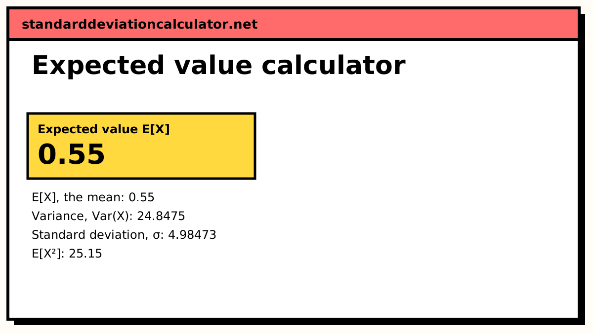
Var(X) = 0.7875 Check: E[X²] = 0·0.5 + 1·0.3 + 4·0.15 + 9·0.05 = 1.35, 1.35 − 0.75² = 0.7875 σ = √0.7875 ≈ 0.8874 defects
Look at the last column. The rare 3-defect batches (5% of the time) contribute almost as much variance as the common zero-defect batches, because their squared distance from the mean is nine times larger. That is typical: the tails of a distribution drive its standard deviation. The expected value calculator runs this table for any outcomes and probabilities you enter, and the variance of a probability distribution section compares it with the data formula.
Continuous random variables
For a continuous variable with density f(x), sums become integrals:
μ = ∫ x·f(x) dx Var(X) = ∫ (x − μ)²·f(x) dx = ∫ x²·f(x) dx − μ²
For a uniform distribution on [a, b], the density is 1/(b − a), the mean is (a + b)/2, and the integral works out to Var(X) = (b − a)²/12, so
σ = (b − a) / √12
If a bus is equally likely to arrive at any moment in the next 10 minutes, the waiting time has mean 5 minutes and σ = 10/√12 ≈ 2.8868 minutes. The uniform distribution calculator handles other intervals.
Shifting and scaling: Var(aX + b)
E[aX + b] = aμ + b Var(aX + b) = a²·Var(X) σ(aX + b) = |a|·σ
Adding a constant moves every outcome by the same amount and leaves the spread alone. Multiplying stretches it. If each defect costs $40 to fix and every batch has a fixed $15 inspection charge, the cost is 40X + 15: mean 40 × 0.75 + 15 = $45, standard deviation 40 × 0.8874 ≈ $35.50. The $15 does not appear in the standard deviation at all. The absolute value matters for negative a: −X has the same standard deviation as X.
Sums and averages: variances add, standard deviations do not
For independent X and Y:
Var(X + Y) = Var(X) + Var(Y) σ(X + Y) = √(σ_X² + σ_Y²)
The total of two dice has variance 35/12 + 35/12 = 35/6 and standard deviation √(35/6) ≈ 2.4152, not 1.7078 + 1.7078 = 3.4157. Some high rolls on one die are offset by low rolls on the other, so the spread grows more slowly than the total. The same rule gives Var(X − Y) = Var(X) + Var(Y): subtracting independent variables still adds their variances.
For the average of n independent copies of X, the variance of the sum is n·σ², and dividing the sum by n divides the variance by n²:
σ(X̄) = σ / √n
The average of four dice has standard deviation 1.7078/√4 ≈ 0.8539; the average of 25 dice, 1.7078/5 ≈ 0.3416. This is the standard error, and the standard error calculator applies it to sample data. Independence matters: for correlated variables a covariance term enters, which is how portfolio standard deviation is built.
Mean and standard deviation of common distributions
| Distribution | Mean μ | Standard deviation σ | Calculator |
|---|---|---|---|
| Bernoulli(p) | p | √(p(1 − p)) | – |
| Binomial(n, p) | np | √(np(1 − p)) | Binomial |
| Poisson(λ) | λ | √λ | Poisson |
| Geometric(p), trials to first success | 1/p | √(1 − p) / p | Geometric |
| Uniform(a, b) | (a + b)/2 | (b − a)/√12 | Uniform |
| Exponential(rate λ) | 1/λ | 1/λ | Exponential |
| Normal(μ, σ) | μ | σ | Normal |
Two quick readings. Ten fair coin flips (binomial, n = 10, p = 0.5) give a head count with mean 5 and σ = √2.5 ≈ 1.5811. A Poisson count averaging 4 per hour has σ = 2. The binomial row is the Bernoulli row summed n times, which is the additivity rule above at work. If you count failures before the first success rather than trials, the geometric mean becomes (1 − p)/p but the standard deviation stays √(1 − p)/p.
Where the sample standard deviation fits
In practice you rarely know the distribution. You observe values and compute the sample standard deviation s, which estimates σ. Roll a real die 20 times and s will land near 1.71 but not on it; roll it 1,000 times and it will usually be within a few hundredths. The n − 1 in the sample formula exists because the sample mean, not μ, sits in the middle of the deviations; the sample vs population guide explains why. With n − 1, s² is an unbiased estimate of σ², though s itself runs slightly low on average.
Chebyshev's inequality: a guarantee for any distribution
Knowing only μ and σ, you can bound how much probability lies far from the mean, whatever the shape of the distribution:
P(|X − μ| ≥ kσ) ≤ 1/k²
At k = 2, at least 75% of the probability lies within two standard deviations of the mean. For the total of two dice (μ = 7, σ ≈ 2.4152) that interval runs from about 2.17 to 11.83, which covers every total from 3 to 11: 34 of the 36 outcomes, or 94.4%. The guarantee holds but is loose, as it must be to cover every distribution. When the variable is close to normal, the tighter 68–95–99.7 rule applies instead. The Chebyshev's theorem calculator works out the bound for any k.
Related calculators
-
Expected value calculator
Enter outcomes and probabilities to get μ, the variance and σ.
-
Binomial distribution calculator
Probabilities plus the mean np and SD √(np(1 − p)).
-
Standard error calculator
The σ/√n rule applied to a sample mean.
-
Chebyshev's theorem calculator
The minimum share within k standard deviations, for any distribution.
Common questions
How do you find the standard deviation of a random variable?
Find the mean μ = Σ x·P(x), then the variance Var(X) = Σ (x − μ)²·P(x), then take the square root. The shortcut Var(X) = E[X²] − μ² gives the same answer with less arithmetic. For a fair die, μ = 3.5, E[X²] = 91/6, Var(X) = 35/12 and σ ≈ 1.7078.
Why is there no n − 1 in the formula for a random variable?
Because nothing is being estimated. The probabilities describe the whole distribution and already sum to 1, so they do the averaging. The n − 1 correction exists only when you estimate σ from a sample and have used the same sample to estimate the mean.
What is the standard deviation of the sum of two dice?
Each die has variance 35/12. The dice are independent, so the variances add to 35/6, and the standard deviation is √(35/6) ≈ 2.4152. Adding the two standard deviations (1.7078 + 1.7078 = 3.4157) overstates it by about 41%.
Can a random variable have a mean but no standard deviation?
Yes. If E[X²] is infinite, the variance is infinite and σ does not exist, even though the mean can be finite. A Student t distribution with 2 degrees of freedom has mean 0 and infinite variance. The Cauchy distribution has neither a mean nor a variance.
Is the standard deviation of a random variable the same as the sample standard deviation?
No. σ is a fixed property of the distribution; the sample standard deviation s is computed from observed values and changes from sample to sample. s is an estimate of σ, and it gets closer as the sample grows. Roll a die 1,000 times and s will usually land within a few hundredths of 1.7078.