Sampling distribution of the sample proportion calculator
Enter the population proportion and the sample size to get the sampling distribution of p̂: its mean, standard error, whether the normal approximation holds, and the probability that the sample proportion falls in a range.
Decimal, fraction or percentage.
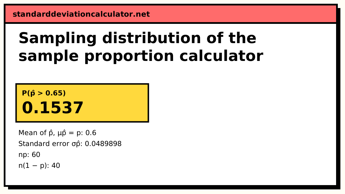
The distribution of p̂ over repeated samples of 100: centre 0.6, standard error 0.04899. Shaded: P(p̂ > 0.65) = 0.1537.
| Range | p̂ from | p̂ to | Share of samples |
|---|---|---|---|
| ±1 SE | 0.551 | 0.649 | 68.27% |
| ±2 SE | 0.502 | 0.698 | 95.45% |
| ±3 SE | 0.453 | 0.747 | 99.73% |
Show the working, step by step
The mean of the sample proportion equals the population proportion.
μp̂ = p = 0.6
Its standard error:
σp̂ = √(p(1 − p) ÷ n) = √(0.6 × 0.4 ÷ 100) = √0.0024 = 0.0489898
Check the success–failure condition for the normal shape.
np = 100 × 0.6 = 60, n(1 − p) = 100 × 0.4 = 40 (both ≥ 10)
Standardise the value(s):
z = (0.65 − 0.6) ÷ 0.0489898 = 1.0206
Probability from the standard normal distribution:
P(p̂ > 0.65) = P(Z > 1.0206) = 1 − 0.846283 = 0.153717
The formulas
μp̂ = p σp̂ = √(p(1 − p) ÷ n) z = (p̂ − p) ÷ σp̂ Normal shape OK when np ≥ 10 and n(1 − p) ≥ 10
The sample proportion is an average of 0s and 1s, so the central limit theorem applies to it just as it does to a sample mean. The population standard deviation of a 0/1 variable is √(p(1 − p)), which is where the numerator comes from.
A worked example
The defaults: 60% of a large population support a proposal (p = 0.6), and you poll a random sample of 100 people. How likely is it that more than 65% of the sample say yes?
- The sampling distribution is centred on μp̂ = 0.6.
- Standard error: √(0.6 × 0.4 ÷ 100) = √0.0024 = 0.04899.
- Condition: np = 60 and n(1 − p) = 40, both at least 10, so the normal model is fine.
- z = (0.65 − 0.6) ÷ 0.04899 = 1.0206.
- P(p̂ > 0.65) = 1 − 0.846283 = 0.1537.
About 15% of samples of 100 would show more than 65% support, even though the true figure is 60%. That is a reminder of how much a sample of 100 can wander: two standard errors either side of 0.6 runs from 0.502 to 0.698, and about 95% of sample proportions land in that range.
Choose "between" with 0.65 and 0.7 and the calculator gives 0.1331, the share of samples with support between 65% and 70%.
What changes the spread
Only two things: p and n. Quadrupling the sample to 400 halves the standard error to 0.0245. Moving p away from 0.5 also narrows it, since p(1 − p) falls. The population size does not appear at all, as long as the sample is a small fraction of it; a poll of 1,000 people is about as precise in a country of 300 million as in a city of 1 million. When the sample is more than about 5% of the population, use the sampling distribution calculator with the finite population correction.
When the condition fails
With p = 0.05 and n = 50, np is only 2.5. The sampling distribution is then lumpy and skewed to the right, and a normal probability can be badly wrong in the tails. The calculator still shows the normal answer but flags it; the binomial distribution calculator gives the exact probability for the count x = n·p̂.
Common mistakes
- Entering percentages as whole numbers. Type 0.65, not 65, for the bound on p̂.
- Using p̂ from your sample in the standard error when the question gives the population p.
- Skipping the success–failure check, especially for rare events.
- Treating 1.96 × σp̂ as a probability. It is a margin; the probability comes from the z-score.
Common questions
What is the sampling distribution of the sample proportion?
It describes how the proportion of successes p̂ = x/n varies from one random sample to the next. Its mean is the population proportion p, its standard deviation (the standard error) is √(p(1 − p)/n), and for large enough samples its shape is approximately normal.
What is the success–failure condition?
A check that the normal approximation is reasonable: the expected number of successes np and of failures n(1 − p) should both be at least 10. Some textbooks use 5 or 15 instead. The condition fails most often when p is close to 0 or 1, because the sampling distribution is then squashed against one end and skewed.
Should I use p or p̂ in the standard error?
Use the population value p when it is known or assumed, as in a probability question or a hypothesis test. When p is unknown and you are building a confidence interval, you have to plug in the sample proportion p̂ instead, and the result is an estimated standard error.
Why does the standard error peak at p = 0.5?
p(1 − p) is largest when p = 0.5, where it equals 0.25. That is why pollsters plan sample sizes with p = 0.5: it gives the widest, most cautious margin. At p = 0.1 the product is only 0.09, so the standard error is 60% of its value at 0.5.
Should I use a continuity correction?
It helps with small samples, because p̂ can only take the values 0, 1/n, 2/n and so on. The correction moves each bound by 1/(2n). With n = 100 that is 0.005, which changes the default answer only slightly. The continuity correction calculator shows the effect on counts.
Related calculators
-
Normal probability for sampling distributions
Probabilities for p̂ or x̄ with the finite population correction.
-
Binomial distribution calculator
Exact probabilities for the number of successes when np is small.
-
Sampling error calculator
The margin of sampling error for a survey proportion.