Normal probability calculator for sampling distributions
Find the probability that a sample mean x̄ or a sample proportion p̂ falls in a range. Enter the population values and the sample size, and add the population size if you are sampling a sizeable share of a finite population.
Decimal, fraction or percentage.
Fill in to apply the finite population correction.
A proportion such as 0.35 or 35%.
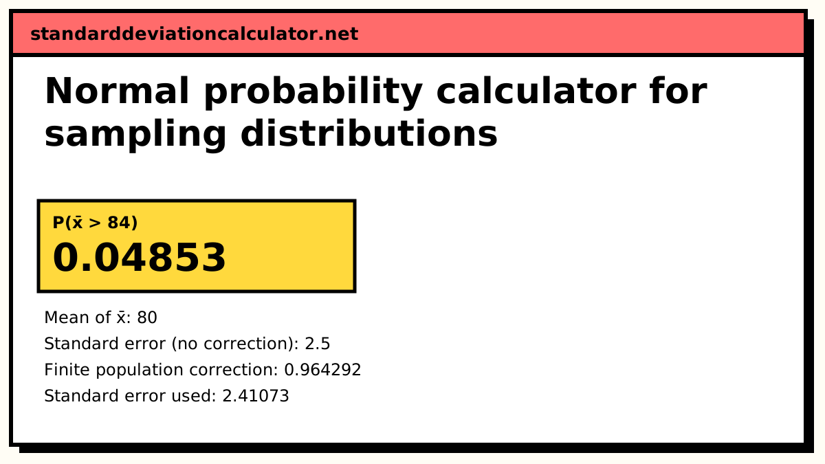
Sampling distribution of x̄: centre 80, standard error 2.411. Shaded: P(x̄ > 84) = 0.04853.
Show the working, step by step
The sampling distribution of x̄ is centred on the population value.
mean = 80
Standard error for an infinite population:
σ ÷ √n = 15 ÷ √36 = 2.5
Sampling without replacement from a finite population reduces the spread by the finite population correction.
FPC = √((N − n) ÷ (N − 1)) = √((500 − 36) ÷ (500 − 1)) = 0.964292 SE = 2.5 × 0.964292 = 2.41073
Standardise with the standard error.
z = (84 − 80) ÷ 2.41073 = 1.6592
Probability from the standard normal table:
P(x̄ > 84) = P(Z > 1.6592) = 1 − 0.951467 = 0.0485329
The formulas
Both statistics have an approximately normal sampling distribution centred on the population value:
Sample mean: x̄ ~ N(μ, σ/√n × FPC) Sample proportion: p̂ ~ N(p, √(p(1 − p)/n) × FPC) FPC = √((N − n) ÷ (N − 1))
When N is not given, the correction factor is 1. Once you have the standard error, the probability comes from a z-score, z = (value − centre) ÷ standard error, and the standard normal distribution.
Worked example: a sample mean from a finite population
The default inputs: a population of N = 500 exam scores has mean μ = 80 and standard deviation σ = 15. A random sample of 36 papers is drawn without replacement. What is the chance the sample mean is above 84?
- Standard error without correction: 15 ÷ √36 = 2.5.
- The sample is 36 ÷ 500 = 7.2% of the population, above the 5% guideline, so apply the correction: FPC = √(464 ÷ 499) = 0.964292.
- Corrected standard error: 2.5 × 0.964292 = 2.41073.
- z = (84 − 80) ÷ 2.41073 = 1.6592.
- P(x̄ > 84) = 1 − 0.951467 = 0.0485.
Without the correction the standard error would be 2.5, z would be 1.6, and the probability 0.0548. The difference is small here, but it grows as the sample takes a larger share of the population. At n = N it would drive the standard error to zero: sample everyone and the mean cannot vary.
Worked example: a sample proportion
Switch the statistic to the sample proportion. Suppose 30% of a large population prefer an option, and you survey 100 people. The chance fewer than 25% of the sample prefer it:
SE = √(0.3 × 0.7 ÷ 100) = 0.045826 z = (0.25 − 0.3) ÷ 0.045826 = −1.0911 P(p̂ < 0.25) = 0.1376
Enter the bounds for p̂ as proportions (0.25), not percentages. If the population had only 2,000 people, the correction factor √(1900 ÷ 1999) = 0.9749 would shrink the standard error to 0.044677 and the probability to 0.1315.
Checking the approximation
For means, the normal shape is safe when the population is roughly normal or n is 30 or more. For proportions, both np and n(1 − p) should be at least 10; the calculator warns when they are not. With a small expected count, work with the exact binomial (or hypergeometric, for a small finite population) distribution instead.
Common mistakes
- Dividing by σ rather than by the standard error when forming the z-score.
- Applying the finite population correction when sampling with replacement. It only applies without replacement.
- Typing 25 for a proportion of 25%. The calculator expects 0.25 for p̂.
- Forgetting that "more than 84" is the upper tail: 1 − Φ(z), not Φ(z).
Common questions
What is a sampling distribution?
The distribution of a statistic, such as a sample mean or sample proportion, over all the samples of size n you could draw. Each sample gives a slightly different value; the sampling distribution describes how those values spread out. Its standard deviation is called the standard error.
When should I use the finite population correction?
When you sample without replacement and the sample is more than about 5% of the population. Each item drawn then tells you a noticeable share of the whole population, so the statistic varies less than σ/√n suggests. The correction factor is √((N − n)/(N − 1)). Leave the population size blank for a very large or effectively infinite population.
Is this different from the central limit theorem calculator?
It uses the same idea but covers more cases: sample proportions as well as sample means, and the finite population correction. The central limit theorem calculator sticks to the mean and also draws the population curve next to the sampling distribution.
Why is my probability different from a textbook answer?
Most often because of rounding. Textbooks round z to two decimals before using a table, so z = 1.6592 becomes 1.66 and the probability 0.04853 becomes 0.04846. The other common cause is whether the book applied the finite population correction.
Can I use this for a sample total instead of a mean?
Yes, with one conversion. A total T = n·x̄, so P(T > t) = P(x̄ > t/n). Divide the total by n and enter it as the value for the sample mean.
Related calculators
-
Central limit theorem calculator
The sampling distribution of the mean drawn against the population.
-
Sampling distribution of p̂
Mean, standard error and the success–failure check for a sample proportion.
-
Z-score calculator
Standardise a single value and find its percentile.