Central limit theorem calculator
Enter the population mean, standard deviation and sample size. The calculator applies the central limit theorem to give the sampling distribution of the mean and the probability that a sample mean lands in the range you choose.
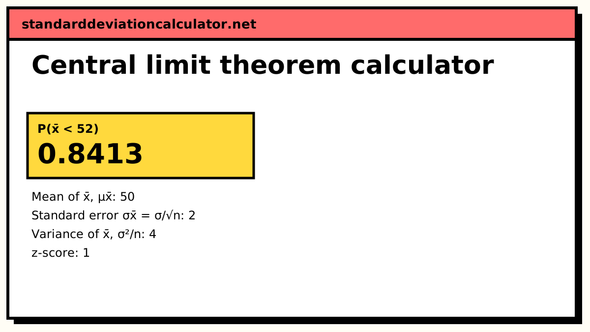
Faint curve: the population, σ = 12. Solid curve: the sampling distribution of x̄ for n = 36, standard error 2. The shaded area is P(x̄ < 52) = 0.8413.
Show the working, step by step
By the central limit theorem, the sample mean is approximately normal with the population mean as its centre.
μx̄ = μ = 50
Its spread is the standard error: σ divided by the square root of the sample size.
σx̄ = σ ÷ √n = 12 ÷ √36 = 12 ÷ 6 = 2
Convert each value to a z-score using the standard error, not σ.
z = (x̄ − μ) ÷ σx̄ = (52 − 50) ÷ 2 = 1
Read the probability from the standard normal distribution.
P(x̄ < 52) = P(Z < 1) = 0.841345
Using σ in place of σ/√n would answer a different question: the chance that one individual value, not the average of n values, falls in the range.
The formula
For samples of size n drawn from a population with mean μ and standard deviation σ, the sample mean x̄ is approximately normally distributed:
x̄ ~ N(μ, σ/√n) μx̄ = μ, σx̄ = σ ÷ √n z = (x̄ − μ) ÷ (σ ÷ √n)
The centre does not move: on average, sample means hit the population mean. The spread shrinks with the square root of the sample size. That √n is why a sample four times larger only halves the standard error.
A worked example
The default inputs describe a population with μ = 50 and σ = 12, sampled 36 at a time. What is the chance that a sample mean comes out below 52?
- The sampling distribution is centred on μx̄ = 50.
- The standard error is σx̄ = 12 ÷ √36 = 12 ÷ 6 = 2.
- Standardise 52 with the standard error: z = (52 − 50) ÷ 2 = 1.
- Read the normal table: P(Z < 1) = 0.8413.
So about 84% of samples of 36 have a mean under 52. Compare that with a single value from the same population: P(X < 52) uses σ itself, z = 2 ÷ 12 = 0.167, and the probability is only 0.566. The value 52 is barely above average for one person but a full standard error above average for a group of 36.
Switch the probability to "between" and enter 48 and 55 to see a two-sided example: the z-scores are −1 and 2.5, and P(48 < x̄ < 55) = 0.9938 − 0.1587 = 0.8351.
Reading the chart
The faint curve is the population, with standard deviation σ. The solid curve is the sampling distribution of x̄, drawn to the same scale: it is √n times narrower and √n times taller, because the same total area of 1 is squeezed into a smaller range. The shaded region is the probability you asked for. Increase n and watch the solid curve tighten while the faint one stays put.
When the answer can be trusted
The calculation assumes the observations in each sample are independent, which holds for random sampling with replacement or from a population much larger than the sample (a common check is n ≤ 10% of the population). When the sample is a sizeable share of a finite population, the spread is smaller than σ/√n; use the sampling distribution calculator, which applies the finite population correction.
The normal shape is exact when the population is normal and approximate otherwise. The calculator warns when n is below 30, since for a skewed population a small sample mean can still be skewed.
Common mistakes
- Using σ instead of σ/√n in the z-score. That answers a question about one value, not about an average.
- Thinking the theorem makes the data normal. It is the distribution of the mean that becomes normal; the individual values keep whatever shape they had.
- Applying it to a tiny sample from a skewed population and trusting the tail probabilities. The tails converge last.
- Confusing the standard error with the margin of error. The margin is the standard error multiplied by a critical value such as 1.96.
Common questions
What does the central limit theorem say?
If you take many random samples of size n from a population with mean μ and standard deviation σ, the sample means form a distribution of their own. The theorem says that distribution is approximately normal once n is large enough, whatever the shape of the population, with mean μ and standard deviation σ/√n.
How large does n need to be?
The usual rule of thumb is n ≥ 30. It is a rough guide, not a threshold. If the population is already normal, any n works. If it is only mildly skewed, 15 to 20 is often enough. For a heavily skewed population, such as incomes or insurance claims, you may need well over 30 before the sample mean looks normal.
What is the difference between σ and σ/√n?
σ measures how much individual values vary. σ/√n, the standard error, measures how much the average of n values varies from sample to sample. With σ = 12 and n = 36 the standard error is 2, so sample means cluster six times more tightly around μ than single values do.
Does the central limit theorem apply to proportions?
Yes. A sample proportion is the mean of a set of 0s and 1s, so it is covered too. Its mean is p and its standard error is √(p(1 − p)/n). The sample proportion calculator works through that case, including the np ≥ 10 check.
What if I only know the sample standard deviation?
Replace σ with s to estimate the standard error. For probabilities about a mean with a small sample and an estimated s, the t distribution is more accurate than the normal; the t-test calculator handles that case.
Related calculators
-
Normal probability for sampling distributions
The same calculation with a finite population correction, for means or proportions.
-
Standard deviation of the sample mean
Just σ/√n, from a standard deviation or from raw data.
-
Normal distribution calculator
Probabilities for a single value from a normal distribution.