Normal approximation calculator
Replace a binomial or Poisson distribution with a normal curve and see how good the swap is. Enter n and p (or λ) and the event, and the calculator gives the normal answer with and without the continuity correction, next to the exact probability.
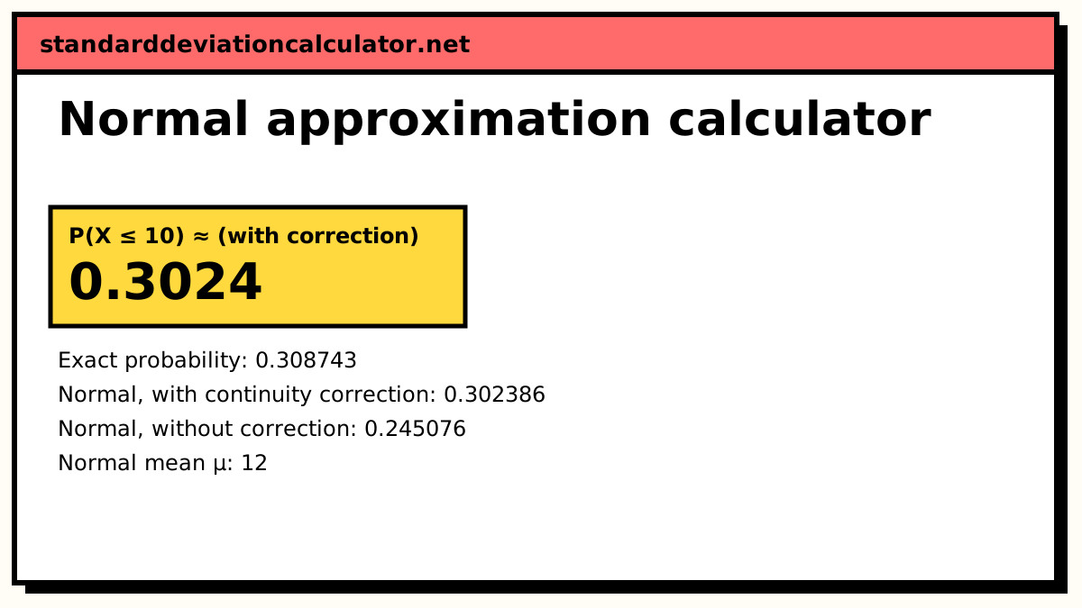
| Method | Statement | Probability | Error vs exact |
|---|---|---|---|
| Exact | P(X ≤ 10) | 0.308743 | – |
| Normal + correction | P(Y < 10.5) | 0.302386 | −0.00636 (−2.06%) |
| Normal, no correction | P(Y < 10) | 0.245076 | −0.0637 (−20.6%) |
Bars: Binomial(n = 40, p = 0.3), with the values counted in P(X ≤ 10) solid. Curve: the normal approximation N(12, 2.898²).
Show the working, step by step
Match a normal to the binomial’s mean and standard deviation.
μ = np = 40 × 0.3 = 12 σ = √(np(1 − p)) = √(12 × 0.7) = 2.89828
With the continuity correction, each whole number k is the interval k − 0.5 to k + 0.5.
P(X ≤ 10) → P(Y < 10.5) z = (10.5 − 12) ÷ 2.89828 = −0.51755 P(Y < 10.5) = 0.302386
Without it, the bound is used as typed.
P(Y < 10) = 0.245076
The exact value sums the probability mass function over the event.
P(X ≤ 10) = 0.308743
The formula
A binomial X ~ B(n, p) is approximated by a normal variable Y with the same mean and standard deviation. For a Poisson with mean λ, the variance is also λ.
Binomial: μ = np, σ = √(np(1 − p)) Poisson: μ = λ, σ = √λ P(X ≤ a) ≈ Φ((a + 0.5 − μ) ÷ σ)
The + 0.5 is the continuity correction: the bar for the value a runs up to a + 0.5, so that is where the normal area should stop. Other inequalities shift the bound in the direction that keeps or drops the boundary value; the continuity correction calculator lists every case.
A worked example
The default: 30% of customers who open a promotional email click through. Out of 40 emails opened, what is the chance that 10 or fewer people click? So X ~ B(40, 0.3) and we want P(X ≤ 10).
First check the rule of thumb: np = 12 and n(1 − p) = 28, both at least 10. Then match the normal:
μ = 40 × 0.3 = 12 σ = √(12 × 0.7) = √8.4 = 2.89828
With the continuity correction, P(X ≤ 10) becomes P(Y < 10.5):
z = (10.5 − 12) ÷ 2.89828 = −0.51755 P(Y < 10.5) = Φ(−0.51755) = 0.302386
Without it, P(Y < 10) = Φ(−0.69007) = 0.245076. The exact binomial probability, summing P(X = k) for k = 0 to 10, is 0.308743.
| Method | Probability | Error |
|---|---|---|
| Exact binomial | 0.308743 | – |
| Normal with correction | 0.302386 | −0.0064 (−2.1%) |
| Normal without correction | 0.245076 | −0.0637 (−20.6%) |
The correction cuts the error by a factor of ten here. That is typical for moderate n: the half unit is a sizeable fraction of σ = 2.9, so leaving it out drops almost the whole bar at X = 10.
How to interpret the output
The headline is the corrected normal probability, because that is the approximation textbooks expect. The table puts all three answers side by side with the absolute and relative error against the exact value. On the chart, the solid bars are the outcomes the event counts and the curve is the normal density drawn on the same scale.
If np or n(1 − p) falls below 10 the calculator warns you and the curve visibly misses the bars. Try n = 10 and p = 0.1 with P(X ≤ 1): the exact value is 0.7361 but the corrected normal gives 0.7009, because the binomial is piled against zero and the normal spills into negative counts.
For a single value, such as P(X = 12), the uncorrected normal gives 0, since a single point has no area under a continuous curve. The corrected version uses the interval 11.5 to 12.5 and gives 0.13697 against an exact 0.13657.
Common mistakes
- Skipping the np ≥ 10 check. With a small or extreme p, the approximation can be badly off even when n looks large.
- Using the variance np(1 − p) where the standard deviation belongs.
- Shifting the bound the wrong way. P(X < 10) excludes 10 and becomes P(Y < 9.5).
- Reporting the approximation as if it were exact. When software is available, quote the exact probability and use the normal only as a check.
Common questions
When can I use the normal approximation to the binomial?
The usual rule is that np and n(1 − p) are both at least 10. Some textbooks accept 5, which is looser. The rule makes sure the binomial is not bunched against 0 or n, where its skew would show. For the default, np = 12 and n(1 − p) = 28, so the rule is met.
What are the mean and standard deviation of the approximating normal?
They are the binomial's own: μ = np and σ = √(np(1 − p)). For a Poisson with mean λ, use μ = λ and σ = √λ. With n = 40 and p = 0.3 that is μ = 12 and σ = √8.4 = 2.89828.
When is the normal approximation to the Poisson reasonable?
When λ is about 10 or more. The Poisson is right-skewed, and the skew fades as λ grows. For λ = 20, P(X ≥ 25) is 0.15677 exactly and 0.15715 by the corrected normal, which is close. Far out in the left tail the match is worse: P(X ≤ 10) is 0.0108 exactly but 0.0168 by the normal.
Why use an approximation when the exact value is easy to compute?
In practice, report the exact value. The approximation still matters because it is how hand calculations and exam questions are done, because it explains why proportions and counts behave normally in large samples, and because many tests (the one-proportion z-test, the sign test for large n) rest on it.
Related calculators
-
Continuity correction
The half-unit rule for every kind of inequality.
-
Binomial distribution
Exact binomial probabilities, mean and standard deviation.
-
Poisson distribution
Exact Poisson probabilities for counts per interval.