Continuity correction calculator
Turn a statement about a count into the right statement about a normal variable. Pick the inequality, enter the value, and the calculator gives the corrected bound. Add n and p (or λ) to get the normal approximation and the exact answer next to it.
Bars: the exact Binomial(n = 100, p = 0.5) probabilities, with the ones counted in P(X ≤ 45) solid. Curve: normal with μ = 50 and σ = 5. Each bar spans k − 0.5 to k + 0.5, which is why the correction adds or removes half a unit.
| Discrete | Continuous (corrected) | Why |
|---|---|---|
| P(X = a) | P(a − 0.5 < Y < a + 0.5) | Widen by half a unit each side |
| P(X < a) | P(Y < a − 0.5) | a itself is excluded, so stop half a unit before it |
| P(X ≤ a) | P(Y < a + 0.5) | a is included, so go half a unit past it |
| P(X > a) | P(Y > a + 0.5) | a is excluded |
| P(X ≥ a) | P(Y > a − 0.5) | a is included |
| P(a ≤ X ≤ b) | P(a − 0.5 < Y < b + 0.5) | Both ends included |
| P(a < X < b) | P(a + 0.5 < Y < b − 0.5) | Both ends excluded |
Show the working, step by step
A count X takes whole-number values. Treat each value k as the interval from k − 0.5 to k + 0.5 on the continuous scale.
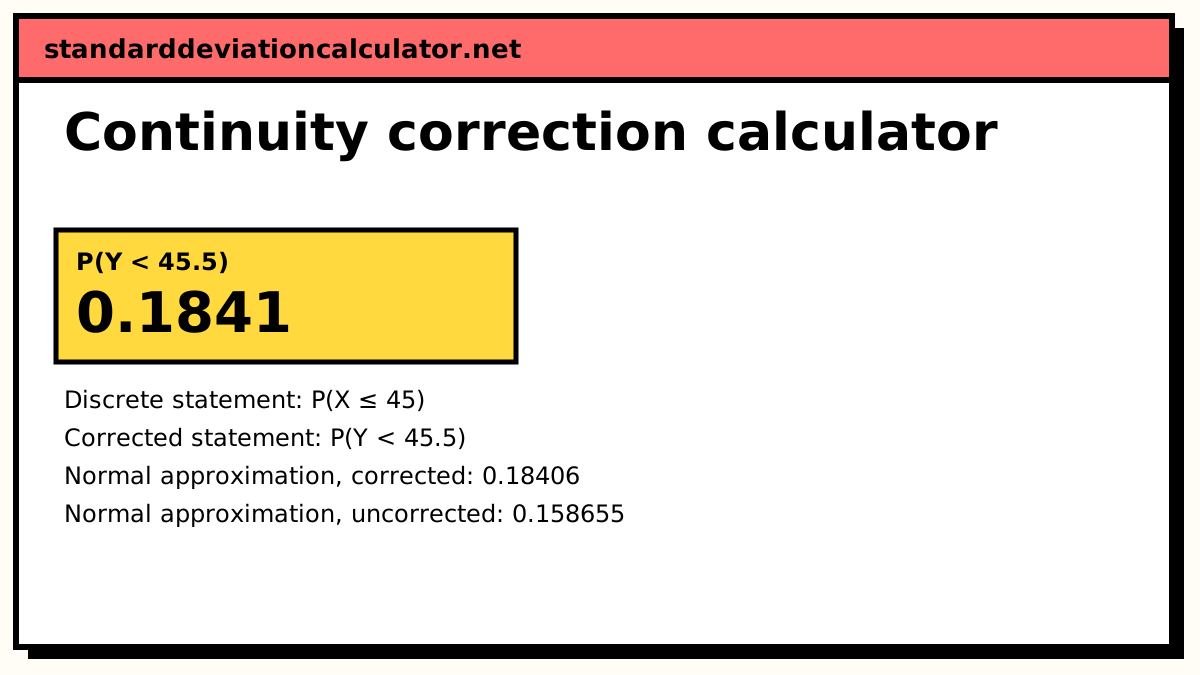
P(X ≤ 45) covers every whole number up to 45
Stretch the event by half a unit at each end that is included.
P(X ≤ 45) → P(Y < 45.5)
Approximate the binomial by a normal with the same mean and standard deviation.
μ = np = 100 × 0.5 = 50 σ = √(np(1 − p)) = √(50 × 0.5) = 5
Standardise the corrected bound(s).
z = (45.5 − 50) ÷ 5 = −0.9
Read the normal probability and compare it with the exact value.
P(Y < 45.5) ≈ 0.18406 Exact P(X ≤ 45) = 0.184101
The rule
A binomial or Poisson variable X only takes whole-number values. Drawn as a bar chart, the bar for the value k runs from k − 0.5 to k + 0.5. A normal variable Y covers those same bars if its boundary sits at the edge of a bar rather than at its centre:
P(X = a) → P(a − 0.5 < Y < a + 0.5) P(X ≤ a) → P(Y < a + 0.5) P(X < a) → P(Y < a − 0.5) P(X ≥ a) → P(Y > a − 0.5) P(X > a) → P(Y > a + 0.5)
A simple way to get it right every time: list the whole numbers the event includes, then go half a unit beyond the lowest and the highest of them. P(X < 45) includes 44 but not 45, so its upper edge is 44.5. P(X ≤ 45) includes 45, so its upper edge is 45.5.
A worked example
The default asks for P(X ≤ 45) when X is the number of heads in 100 tosses of a fair coin, so X ~ Binomial(100, 0.5). The approximating normal has the same mean and standard deviation:
μ = np = 100 × 0.5 = 50 σ = √(np(1 − p)) = √(50 × 0.5) = 5
The event includes 45, so the corrected statement is P(Y < 45.5). Standardise and read the normal table:
z = (45.5 − 50) ÷ 5 = −0.9 P(Y < 45.5) = Φ(−0.9) = 0.18406
The exact binomial probability is 0.184101, so the corrected approximation is off by only 0.00004. Without the correction you would compute P(Y < 45) = Φ(−1) = 0.158655, which is 0.0254 too low: about 14% of the true value. The half unit is what closes that gap.
Switch the statement to P(X < 45) and the bound moves to 44.5, giving 0.13567 against an exact 0.13563. The value 45 itself carries probability 0.0485, and the half-unit shift is how the approximation decides whether to count it.
Reading the result
The headline is the corrected normal probability. Beneath it the calculator shows the uncorrected answer and the exact one, with the error of each. On the chart, the solid bars are the values the event counts and the curve is the normal approximation. Each bar straddles its whole number, so you can see why the cut-off belongs at the bar's edge.
If you only need the corrected bound, perhaps to look up in a table yourself, choose "Nothing, just the corrected bound". The calculator then returns the continuous statement and its limits.
A warning appears when np or n(1 − p) is below 10 (or λ is below 10 for a Poisson). The normal shape is then a poor match for the skewed bars, and no half-unit shift will fully repair that.
Common mistakes
- Moving the bound the wrong way for strict inequalities. P(X > 45) excludes 45, so it becomes P(Y > 45.5), not P(Y > 44.5).
- Correcting both ends of a one-sided event. P(X ≤ 45) has no lower bound to shift.
- Using σ² instead of σ in the z-score. For the binomial, σ is √(np(1 − p)), not np(1 − p).
- Applying the correction to data that are already continuous, such as heights or times. It is only for counts.
- Reporting the approximation when software can give the exact binomial or Poisson value. The approximation is for hand work and for understanding the shape.
Common questions
What is the continuity correction?
An adjustment of half a unit that you make when a normal curve stands in for a count. A count can only be 0, 1, 2 and so on, so each value k is treated as the stretch of the number line from k − 0.5 to k + 0.5. The correction moves the cut-off to the edge of that stretch, so the normal area covers the same values the discrete statement does.
Do I add or subtract 0.5?
Ask whether the boundary value is included. If it is (≤ or ≥), widen the region so it takes in the whole bar for that value: P(X ≤ 45) becomes P(Y < 45.5), and P(X ≥ 45) becomes P(Y > 44.5). If it is excluded (< or >), stop half a unit before it: P(X < 45) becomes P(Y < 44.5). P(X = 45) becomes P(44.5 < Y < 45.5).
When should I use the continuity correction?
Whenever a normal distribution approximates a discrete one: the normal approximation to the binomial, to the Poisson, or to a count-based statistic such as the sign test. It matters most for moderate sample sizes and for probabilities of a single value. When n is in the thousands the half unit is tiny next to the standard deviation and makes little difference.
Why is P(X = k) not zero under the normal approximation?
Under any continuous distribution the probability of one exact point is zero. The correction fixes this by turning the point into an interval one unit wide. For a binomial with n = 100 and p = 0.5, P(X = 45) becomes P(44.5 < Y < 45.5) = 0.04839, against an exact value of 0.04847.
Does the correction always make the answer better?
Usually, for the binomial when np and n(1 − p) are both at least 10. It can make things worse far out in a skewed tail. For a Poisson with λ = 20, P(X ≤ 10) is 0.0108 exactly; the corrected normal gives 0.0168 and the uncorrected one 0.0127. Neither is good there, and the exact value is the one to report.
Related calculators
-
Normal approximation
Compare the corrected and uncorrected normal answers with the exact one.
-
Binomial distribution
Exact binomial probabilities, with no approximation needed.
-
Normal distribution
Areas under any normal curve once you have the corrected bound.