Math
Multivariable calculus calculator
Enter a function of x and y and choose what to find: the gradient, directional derivative and Hessian at a point, all critical points in a region with their type, or a double integral over a rectangle.
Variables x and y. Write products as x*y or x y.
Any non-zero vector; it is scaled to length 1.
Grey lines are level curves of f; the black one passes through the point (2, 1), where f = 3. The ∇f arrow crosses it at right angles, pointing uphill; the u arrow is your direction (arrows show direction, not length).
| ∂/∂x | ∂/∂y | |
|---|---|---|
| ∂f/∂x | 6x | −3 |
| ∂f/∂y | −3 | 6y |
| ∂/∂x | ∂/∂y | |
|---|---|---|
| ∂f/∂x | 12 | −3 |
| ∂f/∂y | −3 | 6 |
Show the working, step by step
The gradient collects the first partial derivatives.
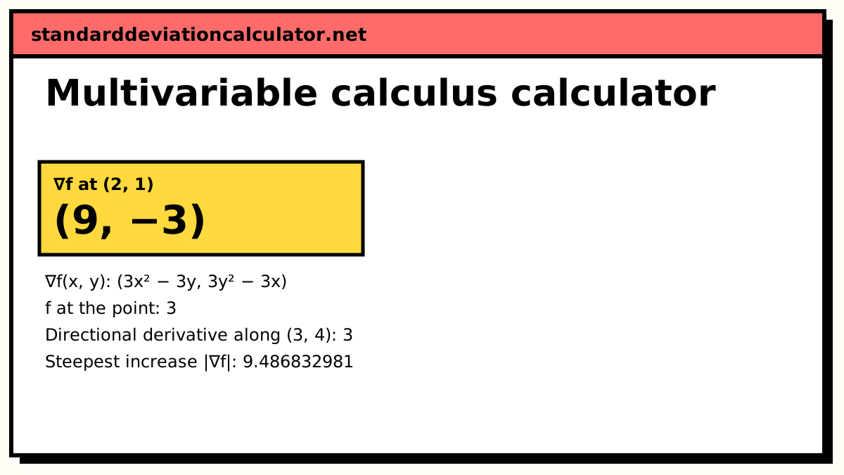
∇f = (∂f/∂x, ∂f/∂y) = (3x² − 3y, 3y² − 3x)
Substitute x = 2, y = 1.
∇f(2, 1) = (9, −3)
Scale the direction to a unit vector.
u = (3, 4) ÷ 5 = (0.6, 0.8)
The directional derivative is the dot product of the gradient with u.
D_u f = 9·0.6 + −3·0.8 = 3
f increases fastest in the direction of ∇f, at rate |∇f|.
|∇f| = √(9² + −3²) = 9.486832981
The Hessian holds the second partials; its determinant at the point is D = fₓₓfᵧᵧ − fₓᵧ².
D = 12·6 − (−3)² = 63
The Hessian only classifies a point when the gradient there is zero; switch to "Critical points" to find those.
The formulas
∇f = (fₓ, fᵧ) D_u f = ∇f · u (|u| = 1) H = [ fₓₓ fₓᵧ ; fᵧₓ fᵧᵧ ] D = fₓₓfᵧᵧ − fₓᵧ² ∬ over [a, b] × [c, d] of f dA = ∫ from a to b [ ∫ from c to d of f(x, y) dy ] dx
A worked example
The default function is f(x, y) = x³ − 3xy + y³, a standard example with one saddle and one minimum.
- Partial derivatives: fₓ = 3x² − 3y and fᵧ = 3y² − 3x.
- At (2, 1): ∇f = (12 − 3, 3 − 6) = (9, −3), and f(2, 1) = 8 − 6 + 1 = 3.
- Direction (3, 4) has length 5, so u = (0.6, 0.8) and D_u f = 9·0.6 − 3·0.8 = 3.
- Second partials: fₓₓ = 6x, fᵧᵧ = 6y, fₓᵧ = −3. At (2, 1) the Hessian is [12, −3; −3, 6], with D = 72 − 9 = 63.
- Critical points: fₓ = 0 gives y = x², then fᵧ = 0 gives x⁴ = x, so x = 0 or 1. At (0, 0), D = 0 − 9 = −9 < 0: a saddle. At (1, 1), D = 36 − 9 = 27 > 0 and fₓₓ = 6 > 0: a local minimum, with f(1, 1) = −1.
- Over the unit square [0, 1] × [0, 1]: ∬ (x³ − 3xy + y³) dA = 1/4 − 3/4 + 1/4 = −1/4.
Reading the second-derivative test
| D | fₓₓ | Critical point is |
|---|---|---|
| > 0 | > 0 | local minimum |
| > 0 | < 0 | local maximum |
| < 0 | any | saddle point |
| = 0 | any | not determined by this test |
D is the determinant of the Hessian, the product of its two eigenvalues. Both positive means the surface curves up in every direction (a bowl); both negative, down in every direction (a cap); opposite signs, up one way and down the other (a saddle).
Double integrals
On a rectangle, integrate the inner variable first with the outer one held fixed, then integrate the result. The calculator tries to do this exactly, showing the intermediate function of x, and always computes the value numerically as well with nested adaptive quadrature. Dividing the integral by the rectangle’s area gives the average value of f over it.
Common mistakes
- Using the direction vector without scaling it to length 1; the result is then |v| times too big.
- Classifying a point from fₓₓ alone. A positive fₓₓ with D < 0 is still a saddle.
- Reading "no critical points found" as proof there are none. The search covers only the region given.
Common questions
What does the gradient tell me?
∇f = (∂f/∂x, ∂f/∂y) points in the direction in which f increases fastest, and its length |∇f| is that fastest rate. It is perpendicular to the level curve through the point. For the default function at (2, 1), ∇f = (9, −3) and |∇f| = √90 ≈ 9.487.
How is the directional derivative calculated?
Scale the direction to a unit vector u, then take the dot product with the gradient: D_u f = ∇f · u. For direction (3, 4), u = (0.6, 0.8), so at (2, 1) the rate is 9·0.6 + (−3)·0.8 = 3. The largest possible value is |∇f|, in the gradient’s own direction.
How does the second-derivative test classify a critical point?
Compute D = fₓₓfᵧᵧ − fₓᵧ² at the point. D > 0 with fₓₓ > 0 is a local minimum, D > 0 with fₓₓ < 0 a local maximum, and D < 0 a saddle point. D = 0 gives no answer: x⁴ + y⁴ has a minimum at the origin and x³ + y³ does not, yet both have D = 0 there.
Can the calculator miss a critical point?
Yes. It solves ∇f = 0 numerically with Newton’s method from a grid of starting points inside the search region. Points outside the region are not looked for, and a function with a whole line of critical points (such as x²y²) gives a sample of points along it. Widen the region if you expect more.
Does the order of integration matter in a double integral?
Not for a continuous function on a rectangle: by Fubini’s theorem, integrating over y then x gives the same value as x then y. The order can matter for how easy the inner integral is, and for regions that are not rectangles the limits change when you swap.
Related calculators
-
Partial derivative
All first and second partials, with Clairaut’s check.
-
Integral
Single integrals, definite and indefinite, with methods named.
-
Derivative
Ordinary derivatives of f(x), rule by rule.
-
Vector calculator
Dot products, magnitudes and unit vectors.
-
Matrix calculator
Determinants and eigenvalues, for example of a Hessian.