Statistics
Sample variance calculator (s²)
Paste a sample of measurements to get its variance, s², computed with the n − 1 denominator that makes it an unbiased estimate of the population variance. The population version is shown beside it in case your data turns out to be the whole group.
Separate numbers with commas, spaces or new lines, or paste a spreadsheet column.
Decimals and negatives are fine; write 10:3 for a value that occurs 3 times.
Your results will appear here: the standard deviation first, then the rest of the summary and a chart.
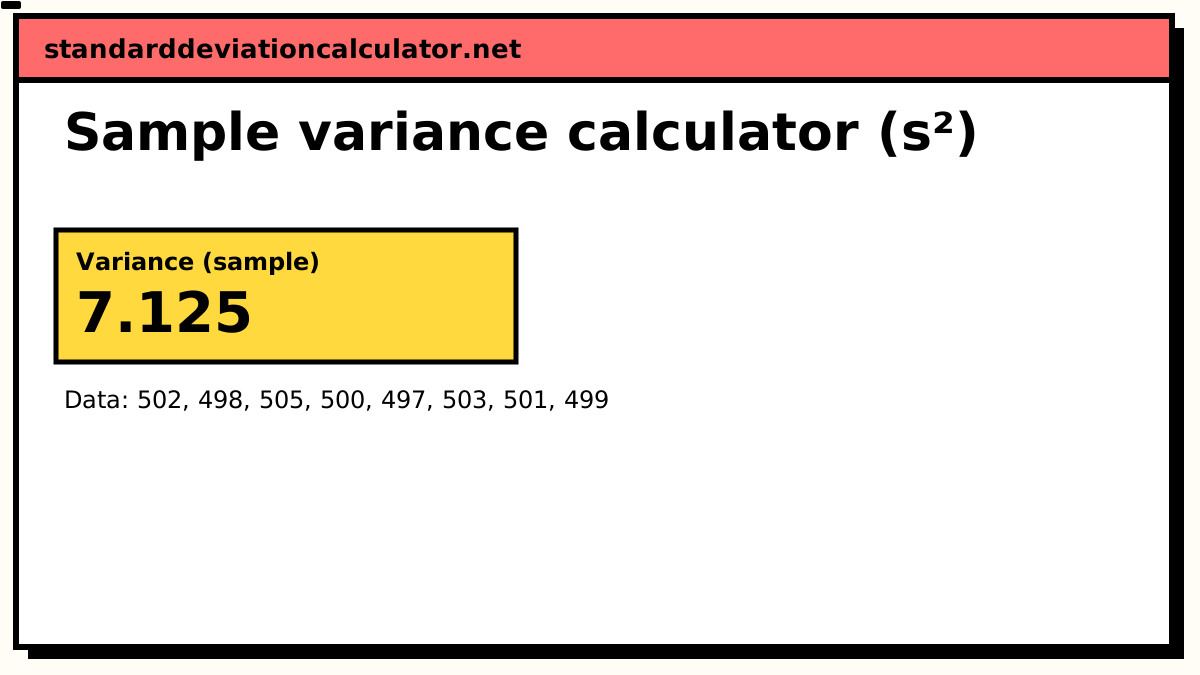
Variance (sample)
7.125
7.12
The variance is in squared units, so it is hard to read on its own. Its square root is the standard deviation, 2.669: your values typically sit about that far above or below their mean of 500.6.
Population variance (σ²): 6.23437, if these values are the whole group.
- Count (n)
- 8
- Mean (x̄)
- 500.625
- Standard deviation (s)
- 2.66927
- Standard error
- 0.943729
- Minimum
- 497
- Q1 (25%)
- 498.75
- Median
- 500.5
- Q3 (75%)
- 502.25
- Maximum
- 505
- Range
- 8
More statistics (5)
- Relative SD (%RSD)
- 0.533187%
- Coefficient of variation
- 0.00533187
- Sum (Σx)
- 4005
- Sum of squares, Σ(x − x̄)²
- 49.875
- IQR (Q3 − Q1)
- 3.5
Data distribution
Shaded bands mark ±1, ±2 and ±3 SD from the mean. 6 of 8 values (75%) fall within ±1 SD.
Chart as text
Mean 500.625, sample standard deviation s = 2.66927, from 8 values between 497 and 505.
- Within ±1 SD (498 to 503.3): 6 of 8 values (75%). About 68% for normal data.
- Within ±2 SD: 8 (100%). About 95% for normal data.
- Within ±3 SD: 8 (100%). About 99.7% for normal data.
Show the working, step by step
The sample variance formula
s² = Σ(x − x̄)² / (n − 1)
x̄ is the sample mean and n the number of values. The numerator is
the sum of squared deviations; the denominator, n − 1, is the number of degrees of
freedom left once the mean has been estimated from the same data. Once you know x̄ and
any n − 1 of the deviations, the last deviation is fixed, because they must sum to zero.
A worked example
A filling line is checked by weighing eight cereal boxes labelled 500 g:
502, 498, 505, 500, 497, 503, 501, 499. These eight are a sample of the
thousands the line fills each shift, so the sample variance is the right statistic.
- Sum = 4005 g over n = 8, so x̄ = 500.625 g.
- Deviations: 1.375, −2.625, 4.375, −0.625, −3.625, 2.375, 0.375, −1.625.
- Squared and added: Σ(x − x̄)² = 49.875 g².
- Divide by n − 1 = 7: s² = 7.125 g².
- The square root gives the sample SD, s = 2.66927 g.
Dividing by 8 instead would give 6.23437 g², about 12% smaller. That gap is the size of the underestimate Bessel's correction repairs, and it shrinks as n grows: at n = 100 the two differ by only 1%.
Why n − 1 makes s² unbiased
The sample mean sits at the exact point that minimises the sum of squared deviations for this sample. The true population mean μ is somewhere else, so deviations measured from it would be larger on average. Algebraically, the expected value of Σ(x − x̄)² is (n − 1)σ², not nσ²:
E[Σ(x − x̄)²] = (n − 1)σ² ⇒ E[s²] = σ²
Averaged over every possible sample, s² hits the population variance exactly. That is what "unbiased" means, and it holds for any distribution with a finite variance, not only the normal.
The standard deviation does not inherit the property. Because √ is concave, E[s] is a little less than √E[s²] = σ. For normal data the shortfall is about 1/(4n): roughly 8% at n = 4 and under 3% at n = 10. For reporting a spread this rarely matters; if you need an unbiased σ for control charts, the tabulated constant c₄ corrects it.
Sample variance in Excel, Sheets, Python and R
| Tool | Sample variance | Watch out for |
|---|---|---|
| Excel / Google Sheets | =VAR.S(A1:A8) | VAR.P divides by n |
| Python (statistics) | statistics.variance(x) | pvariance is the population version |
| NumPy | np.var(x, ddof=1) | the default ddof=0 is the population variance |
| pandas | df['x'].var() | already n − 1 by default |
| R | var(x) | always n − 1; there is no population switch |
NumPy is the usual source of disagreement: np.var(x) on the boxes above returns
6.23437, not 7.125. The Python guide
covers the ddof argument in detail.
When the sample variance is the wrong choice
If your values are the complete group you care about — every employee in a ten-person team, every match a club played this season — there is nothing to estimate, and the population variance is the honest figure. The sample vs population guide walks through borderline cases. For everything else the general variance calculator lets you switch freely.
Related calculators
-
Variance calculator
The general tool, for sample or population variance.
-
Population variance
σ² when your data is the whole group, dividing by N.
-
Sample standard deviation
The square root of s², back in the units of the data.
-
Sample vs population
How to decide which denominator your data needs.
Common questions
What is the sample variance formula?
s² = Σ(x − x̄)² / (n − 1). Subtract the sample mean from each value, square
the differences, add them up, and divide by one less than the number of values.
Why divide by n − 1 and not n?
Because the deviations are measured from the sample mean, which is fitted to the same data. That makes them a little smaller on average than deviations from the true population mean, so dividing by n would underestimate the population variance. Dividing by n − 1 (Bessel's correction) removes that bias exactly.
Is the sample standard deviation unbiased too?
No. s² is an unbiased estimate of σ², but its square root s is slightly biased low as an estimate of σ, because the square root is a curved function. The bias is small — under 3% at n = 10 for normal data — and almost everyone ignores it. The unbiasedness claim belongs to the variance only.
What is the Excel function for sample variance?
=VAR.S(A1:A20). The older VAR is the same function under its
legacy name. VAR.P divides by n and gives the population variance instead.
Can I calculate sample variance with only one value?
No. With n = 1 the denominator n − 1 is zero, so the sample variance is undefined. One observation tells you nothing about spread. The calculator asks for at least two values.