Statistics
Mean and variance calculator
Enter your data to get its mean and variance — the two numbers that describe where a distribution sits and how widely it spreads. The mean appears in the first row of results under the variance, and the working shows how each is built.
Separate numbers with commas, spaces or new lines, or paste a spreadsheet column.
Decimals and negatives are fine; write 10:3 for a value that occurs 3 times.
Your results will appear here: the standard deviation first, then the rest of the summary and a chart.
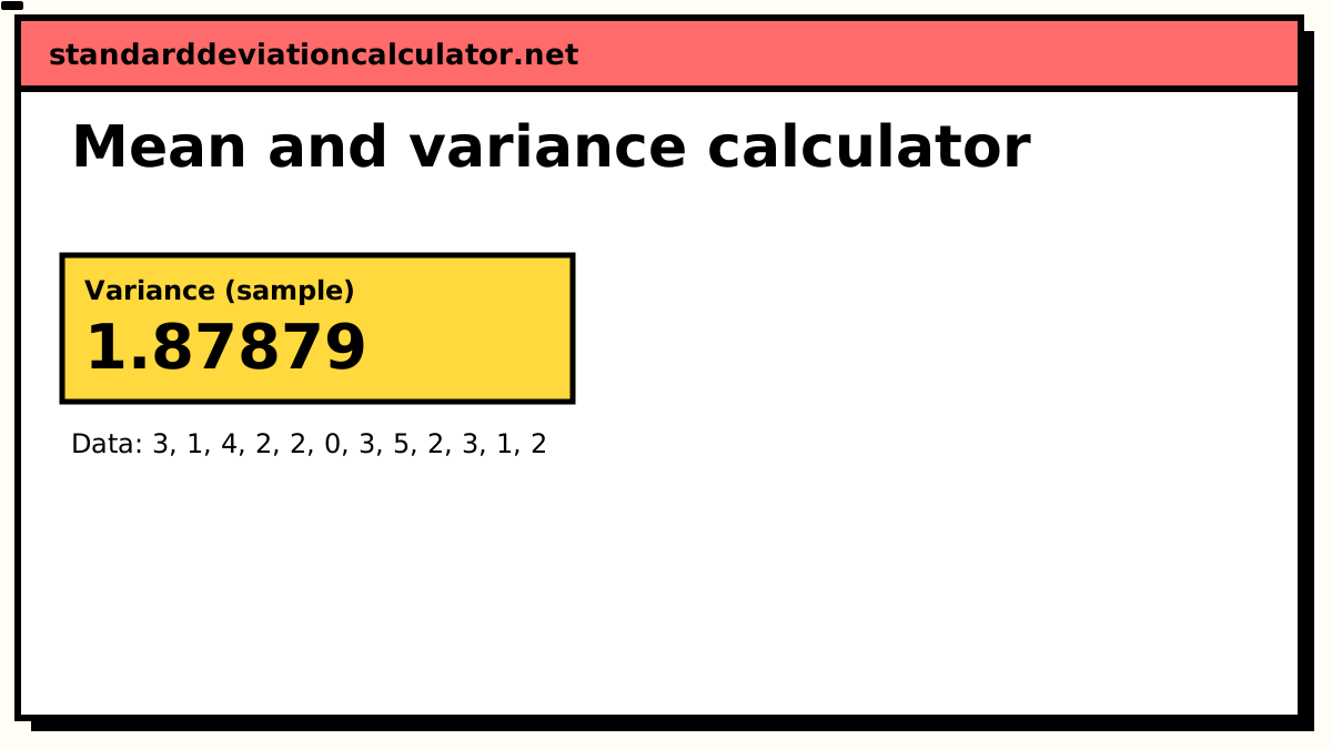
Variance (sample)
1.87879
1.88
The variance is in squared units, so it is hard to read on its own. Its square root is the standard deviation, 1.371: your values typically sit about that far above or below their mean of 2.333.
Population variance (σ²): 1.72222, if these values are the whole group.
- Count (n)
- 12
- Mean (x̄)
- 2.33333
- Standard deviation (s)
- 1.37069
- Standard error
- 0.395684
- Minimum
- 0
- Q1 (25%)
- 1.75
- Median
- 2
- Q3 (75%)
- 3
- Maximum
- 5
- Range
- 5
More statistics (5)
- Relative SD (%RSD)
- 58.7438%
- Coefficient of variation
- 0.587438
- Sum (Σx)
- 28
- Sum of squares, Σ(x − x̄)²
- 20.6667
- IQR (Q3 − Q1)
- 1.25
Data distribution
Shaded bands mark ±1, ±2 and ±3 SD from the mean. 9 of 12 values (75%) fall within ±1 SD.
Chart as text
Mean 2.33333, sample standard deviation s = 1.37069, from 12 values between 0 and 5.
- Within ±1 SD (0.9626 to 3.704): 9 of 12 values (75%). About 68% for normal data.
- Within ±2 SD: 12 (100%). About 95% for normal data.
- Within ±3 SD: 12 (100%). About 99.7% for normal data.
Show the working, step by step
The two formulas
x̄ = Σx / n s² = Σ(x − x̄)² / (n − 1) (sample) σ² = Σ(x − μ)² / N (population)
The mean has to come first, because the variance is measured around it. That order is also why the sample variance divides by n − 1: one degree of freedom has been used up estimating the mean.
A worked example with count data
A help desk logs how many urgent tickets arrive each day for twelve days:
3, 1, 4, 2, 2, 0, 3, 5, 2, 3, 1, 2.
- Σx = 28 tickets over n = 12 days, so the mean is x̄ = 2.33333 tickets per day.
- Squared deviations from 2.33333 add to Σ(x − x̄)² = 20.6667.
- Dividing by n − 1 = 11 gives the sample variance s² = 1.87879.
- The ratio of variance to mean is 1.87879 ÷ 2.33333 = 0.805.
That last ratio is the useful part for counts. A Poisson process — arrivals that happen independently at a steady average rate — has a variance equal to its mean, so a ratio near 1 is what you would expect. Twelve days is not much evidence, but nothing here suggests the tickets arrive in bursts. The Poisson calculator takes λ = 2.33 and gives the probability of any daily count.
Mean and variance as the parameters of a distribution
For the common distributions, knowing the mean and variance either pins the distribution down completely or constrains it tightly:
| Distribution | Mean | Variance | What the pair tells you |
|---|---|---|---|
| Normal N(μ, σ²) | μ | σ² | Everything: the two parameters define the curve |
| Poisson(λ) | λ | λ | They must be equal; a mismatch rules the model out |
| Binomial(n, p) | np | np(1 − p) | Variance is always below the mean |
| Exponential(λ) | 1/λ | 1/λ² | SD equals the mean |
| Uniform(a, b) | (a + b)/2 | (b − a)²/12 | Both follow from the endpoints |
This is the logic of the method of moments: compute the sample mean and variance, then choose the distribution parameters that reproduce them. For a binomial with known n, p = x̄ / n; see the binomial calculator. For a normal model, μ = x̄ and σ² = s² directly, and the normal distribution calculator takes it from there.
Moments beyond the variance
The mean is the first moment and the variance the second central moment. The third central moment, scaled, is the skewness; the fourth is the kurtosis. Two data sets can match on mean and variance and still differ in shape, so if the shape matters, the descriptive statistics calculator reports all four. For variance on its own, use the general variance calculator.
Related calculators
-
Variance calculator
The general variance tool, sample or population.
-
Poisson distribution
The model where the mean and the variance are equal.
-
Binomial distribution
Mean np and variance npq from trials and a probability.
-
Descriptive statistics
The third and fourth moments too: skewness and kurtosis.
Common questions
How do you calculate the mean and variance of a data set?
Add the values and divide by the count for the mean. Then subtract the mean from each value, square the results, add them, and divide by n − 1 (for a sample) or n (for a population) for the variance.
Why are the mean and variance called the first two moments?
The mean is the first moment, E[X]: the average of the values. The variance is the second central moment, E[(X − μ)²]: the average squared distance from the mean. Skewness and kurtosis are built from the third and fourth central moments.
What does it mean if the variance equals the mean?
For count data it is the signature of a Poisson process, where events happen independently at a steady rate. A variance well above the mean (overdispersion) suggests clustering or a rate that changes; well below suggests counts more regular than chance.
What are the mean and variance of a binomial distribution?
Mean np and variance np(1 − p), where n is the number of trials and p the probability of success. Twenty coin flips have mean 10 and variance 5.
Can two data sets have the same mean and variance but look different?
Yes. The mean and variance fix the centre and the spread, not the shape. A symmetric set and a skewed one can share both — which is why a histogram or the skewness is worth a look before assuming normality.