Math
Graphing calculator
Type one to four functions of x and see them on the same axes. The calculator marks every zero and every point where two curves cross, and lists them with their coordinates.
Use x as the variable: ^ for powers, sqrt(x), abs(x), sin, cos, tan, exp, ln or log(x) (natural), log10, pi and e. 2x means 2*x.
f₁(x) = x ^ 2 - 4 f₂(x) = 2 x - 1
| Point | Where | x | y |
|---|---|---|---|
| Zero (x-intercept) | f₁ | -2 | 0 |
| Zero (x-intercept) | f₁ | 2 | 0 |
| Zero (x-intercept) | f₂ | 0.5 | 0 |
| Intersection | f₁ = f₂ | -1 | -3 |
| Intersection | f₁ = f₂ | 3 | 5 |
| x | f₁(x) | f₂(x) |
|---|---|---|
| -5 | 21 | -11 |
| -4 | 12 | -9 |
| -3 | 5 | -7 |
| -2 | 0 | -5 |
| -1 | -3 | -3 |
| 0 | -4 | -1 |
| 1 | -3 | 1 |
| 2 | 0 | 3 |
| 3 | 5 | 5 |
| 4 | 12 | 7 |
| 5 | 21 | 9 |
Show the working, step by step
Read each function. This is how the text was understood (2x means 2 × x):
f₁(x) = x ^ 2 - 4 f₂(x) = 2 x - 1
Sample every function at 2,001 evenly spaced x values from -5 to 5, and join the points. Gaps are left where a function is undefined (a square root of a negative, a division by zero).
Find the zeros: wherever f(x) changes sign between two neighbouring samples, halve the interval repeatedly (bisection) until it is narrower than floating-point precision. A sign change at a vertical asymptote is thrown out, because f does not approach 0 there.
Find the intersections the same way, by solving fᵢ(x) − fⱼ(x) = 0 for each pair of functions.
Check the points by substituting x back in:
f₁(-2) = 0 f₁(2) = 0 f₂(0.5) = 0 f₁ = f₂ at x = -1: y = -3 f₁ = f₂ at x = 3: y = 5
Points are found numerically, to about 10 significant figures. An exact answer such as √2 shows as 1.41421.
What the graph shows
The graph of y = f(x) is every point (x, f(x)). Three kinds of point are usually worth reading off it, and the calculator finds each one numerically:
zero (x-intercept): f(x) = 0 y-intercept: the point (0, f(0)) intersection: f(x) = g(x), i.e. f(x) − g(x) = 0
Finding intersections is the same problem as finding zeros, applied to the difference of two functions. That is how a graph solves equations: to solve x² − 4 = 2x − 1, plot both sides and read the x-coordinates where they cross.
A worked example
The calculator opens with f₁(x) = x² − 4 and f₂(x) = 2x − 1 on −5 ≤ x ≤ 5.
- Zeros of f₁: x² − 4 = 0 gives x = −2 and x = 2.
- Zero of f₂: 2x − 1 = 0 gives x = 0.5.
- Intersections: x² − 4 = 2x − 1 rearranges to x² − 2x − 3 = 0, which factorises as (x − 3)(x + 1) = 0. So x = 3, where y = 2(3) − 1 = 5, and x = −1, where y = 2(−1) − 1 = −3.
- y-intercepts: f₁(0) = −4 and f₂(0) = −1.
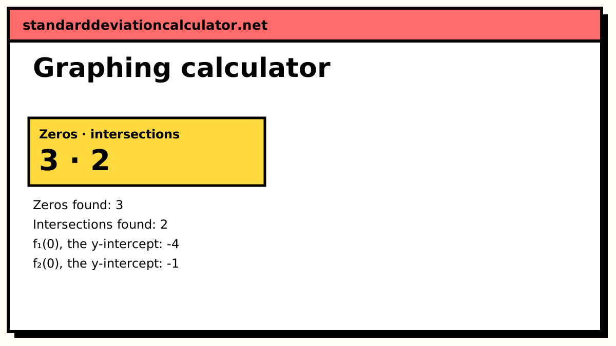
The graph marks the five points (−2, 0), (2, 0), (0.5, 0), (−1, −3) and (3, 5). The headline reads “3 · 2”: three zeros and two intersections.
Functions you can use
| Type | Example | Notes |
|---|---|---|
| Polynomial | x^3 - 3x + 1 | 2x means 2*x |
| Rational | (x + 1)/(x - 2) | Break at the asymptote x = 2 |
| Root | sqrt(x), nthRoot(x, 3) | sqrt is undefined for x < 0 |
| Exponential | exp(x), 2^x, e^(-x) | |
| Logarithm | ln(x), log10(x), log(x, 2) | Defined for x > 0 |
| Trigonometric | sin(x), cos(2x), tan(x) | Radians |
| Absolute value | abs(x - 1) |
Choosing a good window
Most of the trouble with graphs is the window. If a parabola looks like a straight line, the x range is too narrow; if it looks like a thin V, the y range is too tall. Start with the automatic y range, then set it by hand once you know where the interesting part is. For trigonometric functions, a range such as −7 to 7 shows just over two full periods of sin x. For exponentials, keep the range modest: ex at x = 20 is already about 485 million.
Accuracy
The points are found by bisection, which halves the search interval until it reaches the limit of double-precision arithmetic, so zeros and intersections are accurate to roughly ten significant figures. An exact value such as √2 is shown as 1.41421. For an exact answer to a polynomial equation, use the quadratic equation calculator or the polynomial calculator.
Common questions
How do I type functions into the graphing calculator?
Use x as the variable and write the right-hand side of y = …: x^2 - 4,
2x - 1, sin(x)/x, sqrt(x + 3),
exp(-x^2). A leading y = or f(x) = is ignored.
^ is a power, 2x means 2 × x, ln and
log are both the natural logarithm, log10 is base 10, and
pi and e are the constants. Trig functions use radians.
How does it find where two graphs intersect?
Two graphs meet where f(x) = g(x), which is where the difference f(x) − g(x) is zero. The calculator samples the difference at 2,001 points across the x range, finds each place where it changes sign, and narrows each one down by bisection to about ten significant figures. For x² − 4 and 2x − 1 it finds x = −1 and x = 3, the solutions of x² − 2x − 3 = 0.
Why does it miss some zeros?
Only zeros inside the x range are searched, so widen it if you expect roots further out. Two zeros closer together than the sampling gap (the range divided by 2,000) can hide between samples. A root where the curve touches the axis without crossing, as x² does at 0, is caught by a separate check for a minimum of |f| at zero.
What happens at a vertical asymptote?
For a function like 1/x or tan x, the values jump from large negative to large positive across the asymptote. That is a sign change, but not a zero, and the calculator rejects it because |f| does not get small there. The curve is also broken at the jump rather than joined with a vertical line.
Can I set the y range myself?
Yes. Leave both y boxes blank for an automatic range, which ignores the most extreme 2% of values at each end so an asymptote does not flatten the rest of the graph. Fill in both to fix the window, for example −10 to 10 to compare several curves on the same scale.
Related calculators
-
Function calculator
Domain, range and values of a single function.
-
Quadratic equation
Exact roots of ax² + bx + c = 0 with the formula.
-
Trigonometric graphs
Amplitude, period and phase shift of sine and cosine curves.
-
Derivative calculator
Slopes, turning points and the derivative with steps.
-
Linear equation
Solve and graph straight-line equations.