Confusion matrix calculator
Four counts in, every classification metric out. Enter the true and false positives and negatives and the calculator lays out the matrix, each metric with its formula, and the working.
Actual positive, predicted positive.
Actual positive, predicted negative.
Actual negative, predicted positive.
Actual negative, predicted negative.
| Predicted positive | Predicted negative | Total | |
|---|---|---|---|
| Actual positive | TP = 80 | FN = 20 | 100 |
| Actual negative | FP = 10 | TN = 90 | 100 |
| Total | 90 | 110 | 200 |
| Metric | Formula | Value |
|---|---|---|
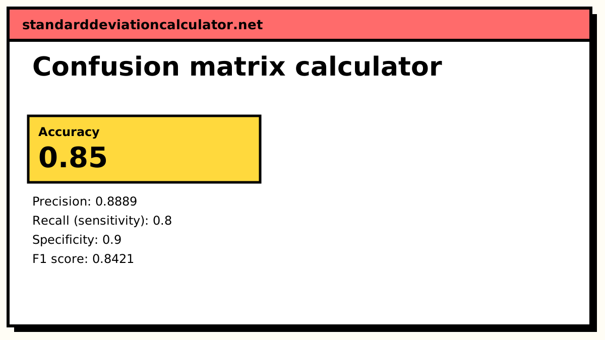
| Accuracy | 0.85 | – |
| Precision (PPV) | 0.8888888888888888 | – |
| Recall / sensitivity (TPR) | 0.8 | – |
| Specificity (TNR) | 0.9 | – |
| F1 score | 0.8421052631578947 | – |
| Negative predictive value | 0.8181818181818182 | – |
| False-positive rate | 0.1 | – |
| False-negative rate | 0.2 | – |
| False discovery rate | 0.1111111111111111 | – |
| Balanced accuracy | 0.8500000000000001 | – |
| Matthews correlation (MCC) | 0.7035264706814484 | – |
| Cohen's kappa | 0.7 | – |
| Youden's J | 0.7000000000000002 | – |
| Prevalence | 0.5 | – |
Show the working, step by step
Totals of the matrix:
n = 80 + 20 + 10 + 90 = 200 actual positives = 100, actual negatives = 100, predicted positives = 90
Accuracy is the share of all cases on the diagonal.
(80 + 90) ÷ 200 = 0.85
Precision divides by the predicted positives, recall by the actual positives.
precision = 80 ÷ 90 = 0.888889 recall = 80 ÷ 100 = 0.8
F1 is the harmonic mean of precision and recall.
F1 = 2 × 80 ÷ (2 × 80 + 10 + 20) = 0.842105
MCC uses all four cells, so it stays honest when the classes are unbalanced.
MCC = (80×90 − 10×20) ÷ √(90×100×100×110) = 0.703526
Kappa compares the observed agreement p₀ with the agreement pₑ expected by chance from the margins.
pₑ = (100×90 + 100×110) ÷ 200² = 0.5 κ = (0.85 − 0.5) ÷ (1 − 0.5) = 0.7
The formulas
accuracy = (TP + TN) ÷ n precision = TP ÷ (TP + FP) recall = TP ÷ (TP + FN) specificity = TN ÷ (TN + FP) NPV = TN ÷ (TN + FN) F1 = 2TP ÷ (2TP + FP + FN) MCC = (TP·TN − FP·FN) ÷ √[(TP + FP)(TP + FN)(TN + FP)(TN + FN)] κ = (p₀ − pₑ) ÷ (1 − pₑ)
The false-positive rate is 1 − specificity and the false-negative rate is 1 − recall. Balanced accuracy is the mean of recall and specificity.
Worked example
The default matrix is a model tested on 200 cases, 100 of each class. It finds 80 of the 100 positives (TP = 80, FN = 20) and wrongly flags 10 of the 100 negatives (FP = 10, TN = 90).
- Accuracy = (80 + 90) ÷ 200 = 0.85.
- Precision = 80 ÷ 90 = 0.8889; recall = 80 ÷ 100 = 0.8; specificity = 90 ÷ 100 = 0.9.
- F1 = 160 ÷ (160 + 10 + 20) = 0.8421, the harmonic mean of 0.8889 and 0.8.
- NPV = 90 ÷ 110 = 0.8182; false-positive rate 0.1; false-negative rate 0.2.
- MCC = (80 × 90 − 10 × 20) ÷ √(90 × 100 × 100 × 110) = 7,000 ÷ 9,949.9 = 0.7035.
- Chance agreement pₑ = (100 × 90 + 100 × 110) ÷ 200² = 0.5, so κ = (0.85 − 0.5) ÷ 0.5 = 0.7.
Balanced accuracy is (0.8 + 0.9) ÷ 2 = 0.85, the same as accuracy because the classes are the same size.
How to interpret the metrics
Choose the metric that matches the cost of each mistake. When missing a positive is expensive (a cancer screen), watch recall. When false alarms are expensive (blocking a customer's card), watch precision or specificity. F1 balances precision and recall but ignores true negatives. MCC and kappa take every cell into account and stay honest when one class is rare; if they are near zero, the model is not doing much better than guessing from the class sizes.
Try changing the default to TP = 5, FN = 5, FP = 5, TN = 185. Accuracy is 0.95, which sounds good, but precision and recall are both 0.5 and MCC is about 0.47. The high accuracy comes mostly from the large negative class.
Common mistakes
- Swapping FN and FP. A false negative is an actual positive the model missed; a false positive is an actual negative it flagged.
- Reading the table the wrong way round. Some software puts predictions in rows and actual classes in columns. Check before you copy the numbers.
- Averaging F1 across folds or classes without saying how. Macro and micro averages can differ a lot.
- Reporting accuracy alone on unbalanced data. Add recall, precision or MCC.
Common questions
What is a confusion matrix?
A 2×2 table that compares a classifier's predictions with the truth. The rows are the actual classes and the columns the predicted ones, giving four counts: true positives (TP), false negatives (FN), false positives (FP) and true negatives (TN). Every standard classification metric is a ratio of these four numbers.
What is the difference between precision and recall?
Precision = TP ÷ (TP + FP): of everything flagged positive, how much was right. Recall = TP ÷ (TP + FN): of everything actually positive, how much was found. A spam filter with high precision rarely junks real mail; one with high recall rarely lets spam through.
When should I use MCC instead of accuracy or F1?
When the classes are unbalanced. The Matthews correlation coefficient uses all four cells and is high only if the model does well on both classes. F1 ignores true negatives entirely, and accuracy can be high just by predicting the majority class. MCC runs from −1 (always wrong) through 0 (no better than chance) to +1 (perfect).
What does Cohen's kappa measure here?
Agreement between predictions and truth beyond what the row and column totals would give by chance. κ = (p₀ − pₑ) ÷ (1 − pₑ), where p₀ is the accuracy and pₑ the agreement expected by chance. Values above about 0.6 are usually read as substantial agreement.
Some metrics show a dash. Why?
A metric is undefined when its denominator is zero. If the model never predicts positive, for example, precision is 0 ÷ 0. The calculator shows a dash and says which count caused it, rather than reporting a misleading 0.
Related calculators
-
Accuracy calculator
Accuracy, balanced accuracy and percent error.
-
Sensitivity and specificity
With Wilson or Clopper–Pearson confidence intervals.
-
Youden's index
J = sensitivity + specificity − 1 and the best cut-off.