Sensitivity and specificity calculator
Enter the four cells of a diagnostic accuracy table. The calculator returns sensitivity, specificity, predictive values and likelihood ratios, each with a confidence interval.
Solid: the test got it right (TP in the first row, TN in the second). Pale: it got it wrong. The solid share of the first row is the sensitivity; of the second, the specificity.
| Test positive | Test negative | Total | |
|---|---|---|---|
| Disease present | TP = 90 | FN = 10 | 100 |
| Disease absent | FP = 30 | TN = 170 | 200 |
| Total | 120 | 180 | 300 |
| Statistic | Formula | Value | 95% CI |
|---|---|---|---|
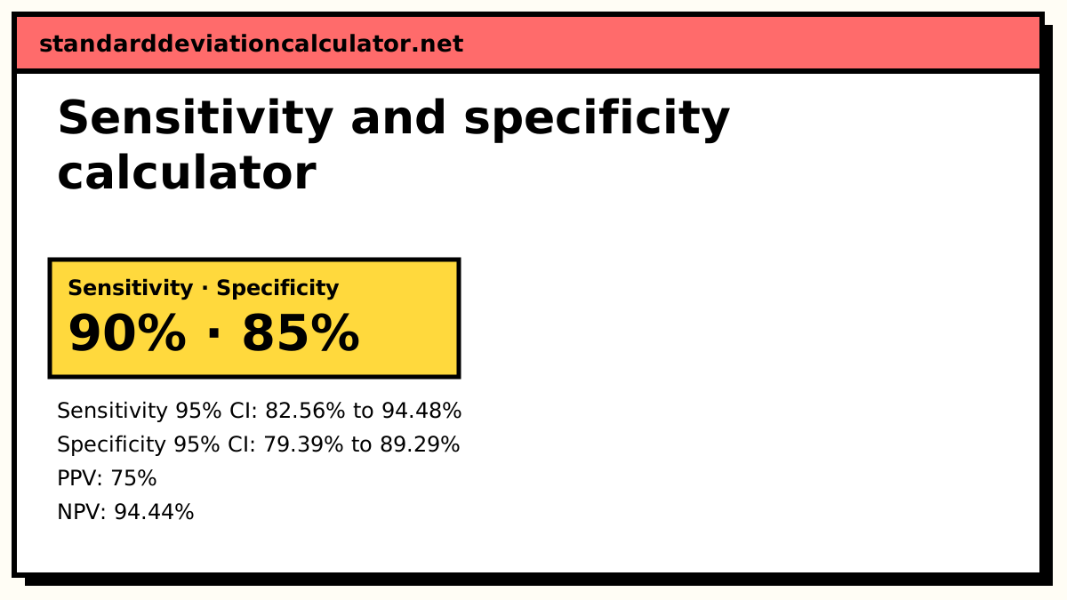
| Sensitivity | TP ÷ (TP + FN) | 90% | 82.56% to 94.48% |
| Specificity | TN ÷ (TN + FP) | 85% | 79.39% to 89.29% |
| Positive predictive value | TP ÷ (TP + FP) | 75% | 66.56% to 81.89% |
| Negative predictive value | TN ÷ (TN + FN) | 94.44% | 90.08% to 96.95% |
| Positive likelihood ratio | sens ÷ (1 − spec) | 6 | 4.286 to 8.399 |
| Negative likelihood ratio | (1 − sens) ÷ spec | 0.1176 | 0.06516 to 0.2124 |
| Accuracy | (TP + TN) ÷ n | 86.67% | 82.35% to 90.05% |
| Prevalence in the sample | (TP + FN) ÷ n | 33.33% | 28.24% to 38.85% |
Show the working, step by step
Sensitivity uses only the people who have the disease (the first row).
sensitivity = 90 ÷ (90 + 10) = 0.9
Specificity uses only the people who do not (the second row).
specificity = 170 ÷ (170 + 30) = 0.85
Predictive values read the table down the columns instead.
PPV = 90 ÷ 120 = 0.75 NPV = 170 ÷ 180 = 0.944444
Likelihood ratios combine sensitivity and specificity.
LR+ = 0.9 ÷ 0.15 = 6 LR− = 0.1 ÷ 0.85 = 0.117647
Wilson limits solve |p̂ − p| = z√(p(1 − p)/n) for p, which behaves well near 0 and 1.
z = 1.95996 centre = (p̂ + z²/2n) ÷ (1 + z²/n), half-width = z/(1 + z²/n) × √(p̂(1 − p̂)/n + z²/4n²) sensitivity: 82.56% to 94.48%
Likelihood-ratio intervals use the log method.
SE(ln LR+) = √(1/TP − 1/(TP + FN) + 1/FP − 1/(FP + TN)) LR+ 95% CI: 4.286 to 8.399
PPV and NPV depend on the prevalence in this sample. If your sample was built with a fixed number of cases and controls, use the post-test probability calculator with the real prevalence instead.
The formulas
sensitivity = TP ÷ (TP + FN) specificity = TN ÷ (TN + FP) PPV = TP ÷ (TP + FP) NPV = TN ÷ (TN + FN) LR+ = sensitivity ÷ (1 − specificity) LR− = (1 − sensitivity) ÷ specificity
Worked example
The default table is a study of 300 people: 100 with the disease and 200 without. The test is positive in 90 of the 100 with disease (TP = 90, FN = 10) and in 30 of the 200 without (FP = 30, TN = 170).
- Sensitivity = 90 ÷ 100 = 90%, 95% Wilson CI 82.56% to 94.48%.
- Specificity = 170 ÷ 200 = 85%, 95% CI 79.39% to 89.29%.
- PPV = 90 ÷ 120 = 75%; NPV = 170 ÷ 180 = 94.44%.
- LR+ = 0.9 ÷ 0.15 = 6, 95% CI 4.29 to 8.40. LR− = 0.1 ÷ 0.85 = 0.118, 95% CI 0.065 to 0.212.
With the Clopper–Pearson method the sensitivity interval widens slightly to 82.38% to 95.10%. The intervals are fairly wide because only 100 people had the disease; to halve their width you need about four times as many cases.
Wilson score interval
For x positives out of n and z = 1.96 at 95% confidence, with p̂ = x/n:
centre = (p̂ + z²/2n) ÷ (1 + z²/n) half-width = [z ÷ (1 + z²/n)] × √(p̂(1 − p̂)/n + z²/4n²)
For sensitivity, p̂ = 0.9 and n = 100: the centre is 0.8852 and the half-width 0.0596, giving 0.8256 to 0.9448. The interval is not symmetric around 0.9 because it is squeezed by the ceiling at 100%.
How to interpret the results
Sensitivity and specificity belong to the test and are the numbers to compare between tests. An LR+ of 6 means a positive result multiplies the odds of disease by six. Starting from a 25% pre-test probability (odds 1 : 3), a positive result takes the odds to 2 : 1, a 67% probability. The post-test probability calculator does that step and draws the Fagan nomogram.
The PPV of 75% here reflects the 33% prevalence in this sample, not the prevalence where the test will be used. In a screening population with 1% prevalence, the same test would have a PPV of about 5.7%.
Common mistakes
- Quoting the PPV from a case-control study as if it applied to patients. Recompute it with the real prevalence.
- Using the Wald interval with small counts or proportions near 100%. It can give limits above 100% or an interval of zero width.
- Putting counts in the wrong cells. The first row is people with the disease; the first column is positive test results.
- Treating a high sensitivity as proof a positive result is correct. That is what PPV and specificity address.
Common questions
What is the difference between sensitivity and specificity?
Sensitivity is the share of people with the condition who test positive, TP ÷ (TP + FN). Specificity is the share of people without it who test negative, TN ÷ (TN + FP). A sensitive test rarely misses a case; a specific test rarely raises a false alarm. The mnemonics SnNout and SpPin say the same: a negative on a highly sensitive test rules out; a positive on a highly specific test rules in.
Why do PPV and NPV change with prevalence but sensitivity does not?
Sensitivity and specificity are calculated within the diseased and non-diseased groups separately, so the size of each group does not matter. PPV and NPV mix the two groups, so they shift as the proportion with the disease changes. The PPV and NPV shown here are only valid for a population with the same prevalence as your sample.
Which confidence interval should I use, Wilson or Clopper–Pearson?
Wilson intervals are close to the stated coverage on average and are the usual recommendation. Clopper–Pearson ("exact") intervals guarantee at least the stated coverage, so they are a little wider and are often required in regulatory submissions. Both behave sensibly near 0% and 100%, unlike the simple Wald interval p ± 1.96√(p(1 − p)/n).
What are likelihood ratios for?
LR+ = sensitivity ÷ (1 − specificity) and LR− = (1 − sensitivity) ÷ specificity say how much a positive or negative result changes the odds of disease. Multiply the pre-test odds by the LR to get the post-test odds. An LR+ above 10 or an LR− below 0.1 is usually a large, often decisive, change.
How are the likelihood-ratio intervals calculated?
On the log scale (Simel, Samsa and Matchar, 1991): SE(ln LR+) = √(1/TP − 1/(TP + FN) + 1/FP − 1/(FP + TN)), and the limits are exp(ln LR ± z × SE). The interval for LR− uses FN and TN in the same way.
Related calculators
-
Post-test probability
Use LR+ or LR− to update a pre-test probability.
-
Confusion matrix calculator
Precision, recall, F1, MCC and kappa.
-
Youden's index
Pick the cut-off that maximises sens + spec − 1.