Statistics
Quartile deviation calculator
Quartile deviation measures the spread of the middle half of a distribution. Enter a list, an (x, f) table or class intervals; the calculator finds Q₁ and Q₃, then the quartile deviation and its coefficient.
Separate with commas, spaces or new lines.
Exclusive classes (10-20, 20-30) or inclusive classes (10-19, 20-29). Inclusive classes are converted to class boundaries.
Grouped (continuous) data always uses the class-interval formula.
| Class | f | cf | Contains |
|---|---|---|---|
| 0-10 | 5 | 5 | |
| 10-20 | 8 | 13 | Q₁ |
| 20-30 | 12 | 25 | |
| 30-40 | 15 | 40 | Q₃ |
| 40-50 | 6 | 46 | |
| 50-60 | 4 | 50 | |
| N | 50 |
Less-than ogive. The marked points are read off at cumulative frequencies 12.5, 37.5.
Show the working, step by step
Add a cumulative frequency (cf) column. N = Σf = 50.
0–10: f = 5, cf = 5 10–20: f = 8, cf = 13 20–30: f = 12, cf = 25 30–40: f = 15, cf = 40 40–50: f = 6, cf = 46 50–60: f = 4, cf = 50
Q₁ class: N/4 = 50/4 = 12.5. The first cumulative frequency ≥ 12.5 is 13, so the Q₁ class is 10–20.
Q₁ = L + ((N/4 − cf) / f) × h = 10 + ((12.5 − 5) / 8) × 10 = 19.375
Q₃ class: 3N/4 = 3 × 50/4 = 37.5. The first cumulative frequency ≥ 37.5 is 40, so the Q₃ class is 30–40.
Q₃ = L + ((3N/4 − cf) / f) × h = 30 + ((37.5 − 25) / 15) × 10 = 38.3333
Quartile deviation: half the interquartile range.
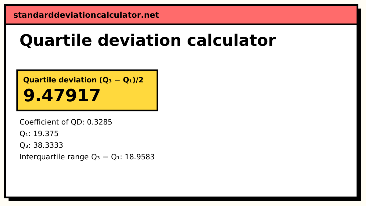
QD = (Q₃ − Q₁)/2 = (38.3333 − 19.375)/2 = 18.9583/2 = 9.47917
Coefficient of quartile deviation: a unit-free ratio for comparing series.
(Q₃ − Q₁)/(Q₃ + Q₁) = 18.9583/57.7083 = 0.3285
L is the lower boundary of the quartile class, cf the cumulative frequency of the class before it, f the frequency of the quartile class and h its width.
The formulas
Quartile deviation QD = (Q₃ − Q₁) / 2 Coefficient of QD = (Q₃ − Q₁) / (Q₃ + Q₁)
The quartiles themselves come from the usual rules: the k(n + 1)/4th item for a list or a
discrete series, and Qₖ = L + ((kN/4 − cf)/f) × h for class intervals. The
quartile calculator explains each rule in detail.
Worked example: continuous series
The calculator opens on this grouped distribution (N = 50):
| Class | f | cf |
|---|---|---|
| 0-10 | 5 | 5 |
| 10-20 | 8 | 13 |
| 20-30 | 12 | 25 |
| 30-40 | 15 | 40 |
| 40-50 | 6 | 46 |
| 50-60 | 4 | 50 |
- Q₁: N/4 = 12.5 falls in 10-20 (cf 13). Q₁ = 10 + ((12.5 − 5)/8) × 10 = 19.375.
- Q₃: 3N/4 = 37.5 falls in 30-40 (cf 40). Q₃ = 30 + ((37.5 − 25)/15) × 10 = 38.333.
- QD = (38.333 − 19.375)/2 = 18.958/2 = 9.479.
- Coefficient of QD = 18.958/(38.333 + 19.375) = 18.958/57.708 = 0.3285.
Worked example: individual series
Switch to an individual series and the default list is
23, 15, 31, 8, 26, 12, 38, 17, 29, 21. Sorted, Q₁ is the 2.75th item, 14.25, and
Q₃ is the 8.25th item, 29.5. So QD = (29.5 − 14.25)/2 = 7.625, and the
coefficient is 15.25/43.75 = 0.3486. With Excel's QUARTILE.INC convention
the quartiles would be 15.5 and 28.25, giving QD = 6.375; the method list lets you match
whichever your course uses.
When to use quartile deviation
Quartile deviation is the natural partner of the median. Use it when the data are skewed, contain outliers, or come in a table with open-ended classes such as “below 10” or “60 and above”, where a mean or standard deviation cannot be calculated honestly. Because it only uses Q₁ and Q₃, a single extreme value has no effect on it.
For symmetric, well-behaved data the standard deviation is more informative, because it uses every observation. For a normal distribution, QD is about 0.6745 times the standard deviation, so the two can be compared roughly: a QD far below two-thirds of the SD suggests heavy tails.
Absolute and relative measures
| Absolute measure | Relative measure (coefficient) |
|---|---|
| Range L − S | (L − S)/(L + S) |
| Quartile deviation (Q₃ − Q₁)/2 | (Q₃ − Q₁)/(Q₃ + Q₁) |
| Mean deviation | MD / mean (or median) |
| Standard deviation σ | σ / x̄ (× 100 gives the coefficient of variation) |
The absolute measures are in the units of the data. The coefficients are pure numbers, so use them whenever you compare two series in different units or with very different averages.
Common mistakes
- Reporting the interquartile range as the quartile deviation. QD is half of it.
- Dividing by 2 in the coefficient. The coefficient is (Q₃ − Q₁)/(Q₃ + Q₁); the halves cancel.
- Using class limits rather than boundaries for inclusive classes (10-19, 20-29). The calculator converts them for you.
Common questions
What is the formula for quartile deviation?
QD = (Q₃ − Q₁) / 2. It is half the interquartile range, which is why it is
also called the semi-interquartile range. Its relative form is the coefficient of quartile
deviation, (Q₃ − Q₁) / (Q₃ + Q₁).
What does the coefficient of quartile deviation tell you?
It is the spread of the middle half of the data relative to the size of the quartiles, with no units. That lets you compare the variability of, say, wages in rupees with heights in centimetres, or two series with very different averages. A higher coefficient means relatively more spread.
Is quartile deviation the same as the interquartile range?
No, it is half of it. For the grouped example on this page the interquartile range is 38.33 − 19.375 = 18.96, and the quartile deviation is 9.48.
What are the merits and limitations of quartile deviation?
It is easy to calculate, is not affected by extreme values, and works with open-ended classes because it only needs the middle half of the data. On the other hand it ignores the lowest 25% and highest 25% of observations entirely, and it does not lend itself to further algebra the way the standard deviation does.
Can the coefficient of quartile deviation be more than 1?
Not for data that are all positive: Q₃ − Q₁ is always smaller than Q₃ + Q₁ when Q₁ is above zero. If Q₁ is negative the ratio can exceed 1 or become meaningless, so the coefficient is only used for positive quantities.
Related calculators
-
Quartile calculator
Q1, Q2 and Q3 with the working for each.
-
Decile deviation
The same idea using D1 and D9: the middle 80%.
-
Mean deviation
Average distance from the mean, median or mode.
-
Coefficient of range
The simplest relative measure of spread.
-
IQR calculator
The interquartile range and outlier fences.